Below, you can find examples on how to use some of the core functions of the hibiiscus package.
First, we show how to create a hibiiscus database (based on simulated data).
We then show various ways in which a hibiiscus database object can be manipulated, for example filtering to remove particular sites, or realigning land-use variables. We follow this by saving the hibiiscus database for future use.
Next, diversity metrics for each site (and between sites) will be calculated, before fitting mixed-effects models using
lme4.We then demonstrate the use of cross-validation to interrogate model performance.
BAnd run model projection, including estimation of the Area of Applicability (AOA, see Meyers and Pebesma, 2021).
Before finishing with an example of model fitting integrating two datasets. ### 1. Load package and PREDICTS-like data
# Load our simulated data - and assign the dataset an identifying name.
hib_db <- hib_create_db(path_species = system.file("extdata", "dummy_species_rc.rds",
                                                   package = "hibiiscus", mustWork = TRUE),
                       dataset_name = "Dummy data")
#>
#> Initialising HibDatabase using Dummy data data ...
#>
#> Generating sites dataframe...
#>

# View a summary of the hib database object
print(hib_db)
#> Hibiiscus database (including dataset/s: Dummy data)
#> Last updated: 2026-10-30 21:59:50.365968
#>   Number of sites:               200
#>   Number of species:             873
#>   Number of taxa (orig. names):  873
#>   Land use (class x intensity):  4 x 3
#>   LU/I legend sourced from:      Original LU/I legend.
#>   Database updates:              NA
#>
#>   Effort-correction applied:     FALSE
#>   Filtering conducted:           NA
#>   Data columns added:            NA
#>
#>   Within-site diversity metrics calculated:   NA
#>   Between-site diversity metrics calculated:  NA
#>   Site-site contrast metrics calculated:      NA
# The default plot function generates a map of sites within the dataset.
hib_db$plot()
#> Warning: `label` cannot be a <ggplot2::element_blank> object.
#> `label` cannot be a <ggplot2::element_blank> object.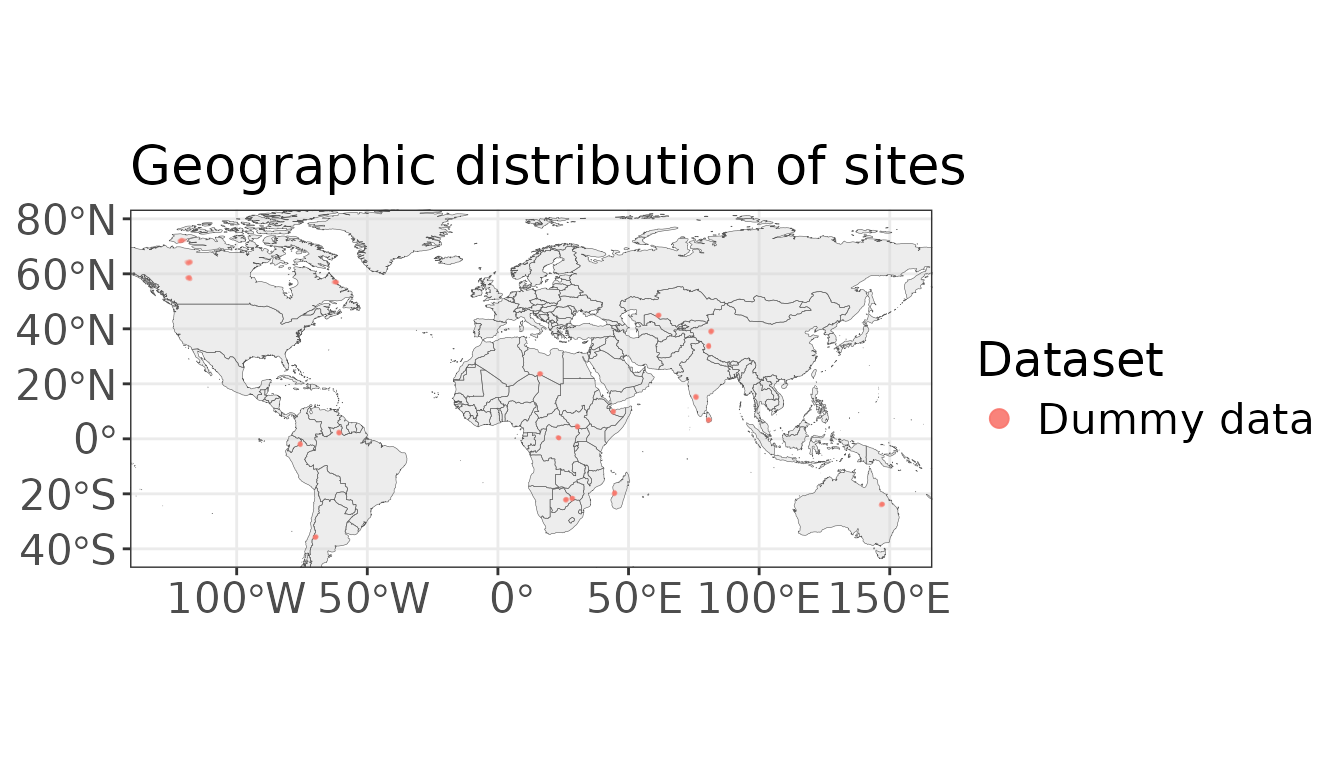
2. Filter data to remove sites in Oceania
hib_db <- hib_filter_sites(hib_db,
                           UN_region != "Oceania")
#>
#> Filtering HibDatabase using: UN_region != 'Oceania' ...
#>
# Plot the sites within the filtered dataset.
hib_db$plot()
#> Warning: `label` cannot be a <ggplot2::element_blank> object.
#> `label` cannot be a <ggplot2::element_blank> object.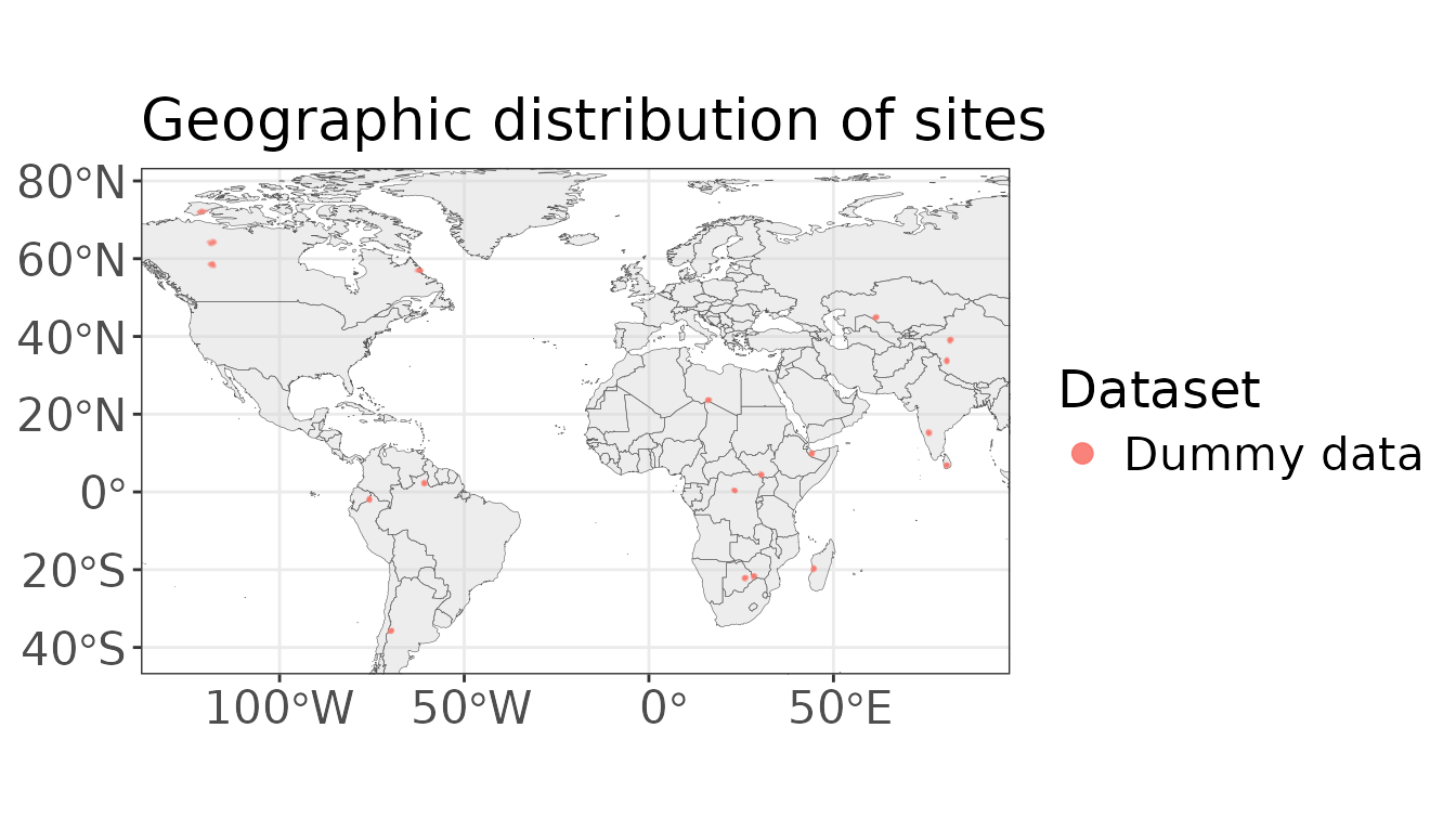
3. Condense land-use categories
Here, we will add a new land-use ‘legend’ to the database, grouping original land-use types into “Natural”, “Semi-natural” and “Human”.
# Make alt_lu_leg using SSBS, Predominant_land_use - re-align to c("Natural", "Semi-natural", "Human")
alt_lu_df <- hib_db$sites[,c("SSBS", "Predominant_land_use")] |>
  dplyr::mutate(Predominant_land_use = dplyr::case_when(Predominant_land_use == "Primary" ~ "Natural",
                                                        Predominant_land_use == "Secondary" ~ "Semi-natural",
                                                        T ~ "Human"),
                Predominant_land_use = factor(Predominant_land_use,
                                              levels = c("Natural", "Semi-natural", "Human")),
                Use_intensity = "",
                LUI = Predominant_land_use)

# Make an lu legend
alt_lu_leg <- hib_create_lu_legend(alt_lu_df)
#>
#> Initialising HibLULegend from data.frame: alt_lu_df...
#>

# Set the lu legend on the database
hib_db <- hib_set_lu_legend(hib_db, alt_lu_leg)
#>
#> Setting land-use legend for HibDatabase...
#>
#> Joining with `by = join_by(SSBS)`
#> Joining with `by = join_by(SSBS)`

# Save the database object for future use
# save_hib(hib_db,
#          "../Data/example_hib.rds")
4. Correct measurements for sampling effort, calculate total abundance per site and Bray-curtis dissimilarity between sites (within studies).
hib_db$hib_effort_correction()
#>
#> Correcting biodiversity measurements for sampling effort ...
#>

# Biodiversity metric calculations
hib_db <- hib_calc_div_within(hib_db,
                              c("Total_abundance"))
#>
#> Calculating within-site biodiversity metrics ...
#>
#>     Total abundance ...
#>
hib_db <- hib_calc_div_between(hib_db,
                              c("baselga_bray_balanced"),
                              baseline_lui = "Natural")
#>
#> Preparing site-contrasts to calculate compositional dissimilarity ...
#>
#> 351 site comparisons to make ...
#>
#> Calculating compositional dissimilarity ...
#>
#>     Non-vegan dissimilarity metrics (Baselga_bray_balanced) ...
#>

# And calculate site contrasts too (for between site models)
hib_db <- hib_calc_site_contrasts(hib_db,
                                  c("lui_contrast"),
                                  baseline_lui = "Natural")
#>
#> Collating data for site contrasts...
#>
#>     351 site comparisons to make...
#>
#> Calculating site contrasts...
#>
#>     (LUI_contrast) ...
#>


print(hib_db)
#> LUI contrast
#> Hibiiscus database (including dataset/s: Dummy data)
#> Last updated: 2026-10-30 22:00:00.181869
#>   Number of sites:               190
#>   Number of species:             868
#>   Number of taxa (orig. names):  868
#>   Land use (class x intensity):  3 x 1
#>   LU/I legend sourced from:      data.frame ('alt_lu_df')
#>   Database updates:              NA
#>
#>   Effort-correction applied:     TRUE
#>   Filtering conducted:           1: UN_region != 'Oceania'
#>   Data columns added:            NA
#>
#>   Within-site diversity metrics calculated:   Total abundance
#>   Between-site diversity metrics calculated:  Baselga bray balanced
#>   Site-site contrast metrics calculated:      LUI contrast
Note: other metrics of within-site diversity include; “Species_richness”, “Chao1_diversity”, “Rarefied_species_richness”, “Simpson_diversity”, “Shannon_diversity”, “Mean_abundance”, “Geometric_mean_abundance”, “HillShannon_diversity”, “HillSimpson_diversity”, “Evenness”, “PIE” and “Equalness”.
Other metrics of between-site diversity include; “manhattan”, “euclidean”, “canberra”, “clark”, “bray”, “kulczynski”, “jaccard”, “gower”, “altGower”, “morisita”, “horn”, “mountford”, “raup”, “binomial”, “chao”, “cao”, “mahalanobis”, “chisq”, “chord”, “hellinger”, “aitchison”, “robust.aitchison”, “hypervolume”, “cosine”, “theta”, “baselga_bray_balanced”, “baselga_bray_gradient”, “baselga_ruzicka_balanced” and “baselga_ruzicka_gradient”.
5. Fit a simple model of (rescaled) total abundance in response to land-use, and a simple model of Bray-Curtis dissimilarity.
# Within-site abundance model
hib_ta_mod <- hib_fit_lme4(hib_db,
                           sqrt(Rescaled_total_abundance) ~ LUI + (1 | SS) + (1 | SSB),
                           REML = F,
                           calc_CIs = "Wald")
#>
#> Collating data for model fitting...
#>
#> Fitting model (this may take some time) ...
#>
#> Collating model details ...
#>
#>     Getting confidence intervals ...
#>
#> Initialising HibModelLME4 object ...

print(hib_ta_mod)
#> Hibiiscus fitted model (lme4)
#> Last updated: 2026-10-30 22:00:00.548822
#>   Number of sites:               190
#>   Number of species:             868
#>   Number of taxa (orig. names):  868
#>
#> --------------------
#>
#> Summary of fitted model
#> Linear mixed model fit by maximum likelihood  ['lmerMod']
#> Formula: sqrt(Rescaled_total_abundance) ~ LUI + (1 | SS) + (1 | SSB)
#>    Data: mod_df
#>
#>       AIC       BIC    logLik -2*log(L)  df.resid
#>      29.2      48.7      -8.6      17.2       184
#>
#> Scaled residuals:
#>      Min       1Q   Median       3Q      Max
#> -1.77106 -0.71163 -0.05377  0.43234  3.11027
#>
#> Random effects:
#>  Groups   Name        Variance Std.Dev.
#>  SS       (Intercept) 0.00510  0.07142
#>  SSB      (Intercept) 0.03934  0.19834
#>  Residual             0.05107  0.22598
#> Number of obs: 190, groups:  SS, 19; SSB, 19
#>
#> Fixed effects:
#>                 Estimate Std. Error t value
#> (Intercept)      0.57336    0.06113   9.380
#> LUISemi-natural  0.01758    0.05165   0.340
#> LUIHuman         0.05399    0.04392   1.229
#>
#> Correlation of Fixed Effects:
#>             (Intr) LUISm-
#> LUISem-ntrl -0.451
#> LUIHuman    -0.528  0.631
#>
#>
#> Performance metrics:
#>  R-squared (marg.)     0.005
#>  R-squared (cond.)     0.468
#>  AIC                  29.189
#>  AICc                 29.648
#>  BIC                  48.671

# Between-site Bray-Curtis model
hib_bc_mod <- hib_fit_lme4(hib_db,
                           car::logit(Baselga_bray_balanced, adjust = 0.001, percents = FALSE) ~ LUI_contrast + (1 | SS),
                           REML = F,
                           calc_CIs = "Wald",
                           # Ensure Natural_vs_Natural is the baseline/intercept
                           relevel_specs = c("LUI_contrast" = "Natural_vs_Natural"))
#>
#> Collating data for model fitting...
#>
#> Fitting model (this may take some time) ...
#>
#> Registered S3 method overwritten by 'car':
#>   method           from
#>   na.action.merMod lme4
#> Collating model details ...
#>
#>     Getting confidence intervals ...
#>
#> Initialising HibModelLME4 object ...

print(hib_bc_mod)
#> Hibiiscus fitted model (lme4)
#> Last updated: 2026-10-30 22:00:00.613004
#>   Number of sites:               170
#>   Number of species:             814
#>   Number of taxa (orig. names):  814
#>
#> --------------------
#>
#> Summary of fitted model
#> Linear mixed model fit by maximum likelihood  ['lmerMod']
#> Formula: car::logit(Baselga_bray_balanced, adjust = 0.001, percents = FALSE) ~
#>     LUI_contrast + (1 | SS)
#>    Data: mod_df
#>
#>       AIC       BIC    logLik -2*log(L)  df.resid
#>      45.3      64.6     -17.6      35.3       346
#>
#> Scaled residuals:
#>     Min      1Q  Median      3Q     Max
#> -3.5714 -0.5917  0.0050  0.5139  3.6248
#>
#> Random effects:
#>  Groups   Name        Variance Std.Dev.
#>  SS       (Intercept) 0.009467 0.0973
#>  Residual             0.060541 0.2461
#> Number of obs: 351, groups:  SS, 17
#>
#> Fixed effects:
#>                                      Estimate Std. Error t value
#> (Intercept)                         -0.008831   0.039933  -0.221
#> LUI_contrastNatural_vs_Human        -0.033874   0.035508  -0.954
#> LUI_contrastNatural_vs_Semi-natural -0.039045   0.041852  -0.933
#>
#> Correlation of Fixed Effects:
#>             (Intr) LUI_N__H
#> LUI_cntN__H -0.696
#> LUI_cnN__S- -0.600  0.644
#>
#>
#> Performance metrics:
#>  R-squared (marg.)     0.003
#>  R-squared (cond.)     0.138
#>  AIC                  45.258
#>  AICc                 45.432
#>  BIC                  64.562
# Check the abundance model
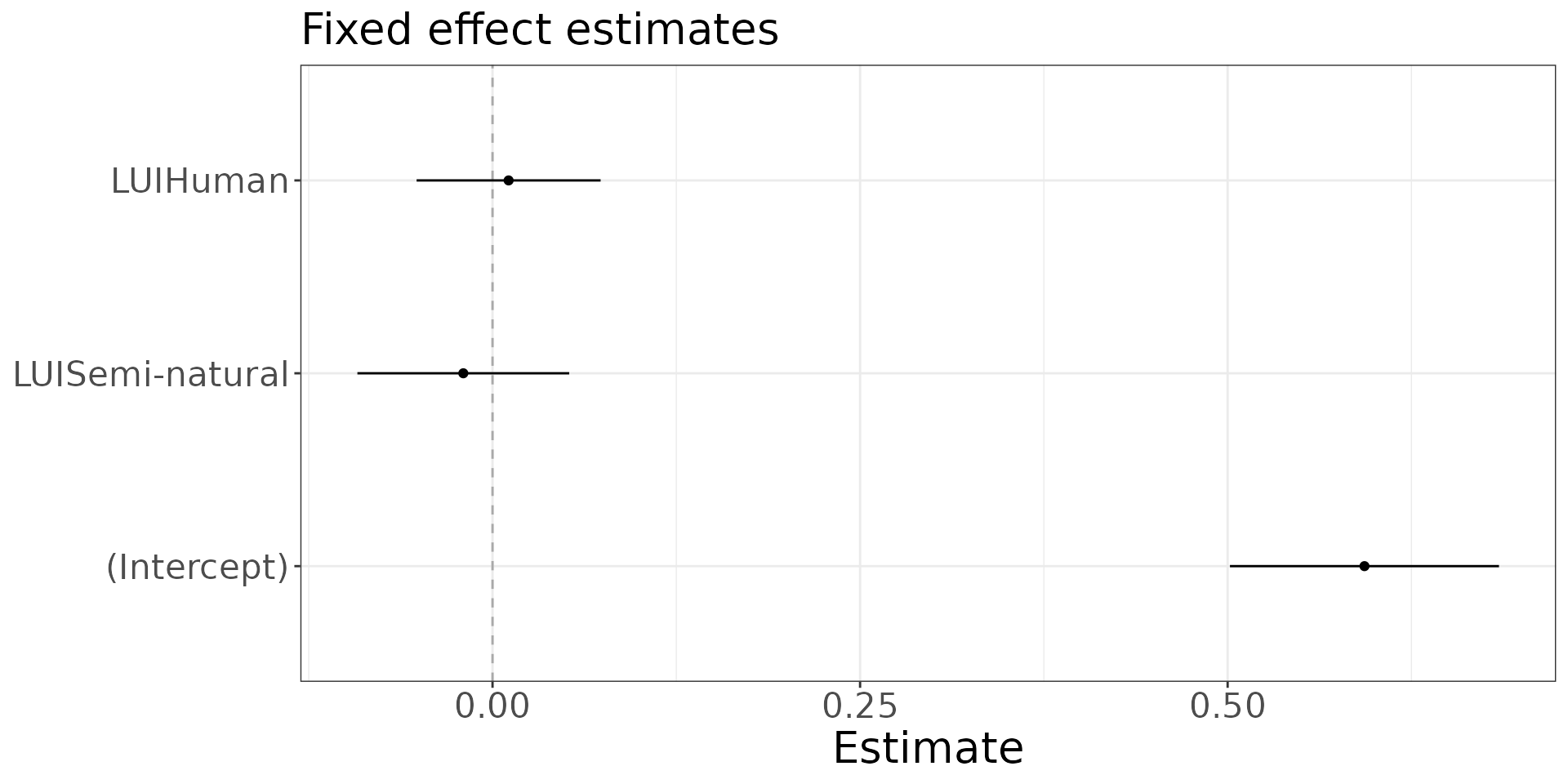
hib_ta_mod$plot()
#> Warning: `label` cannot be a <ggplot2::element_blank> object.

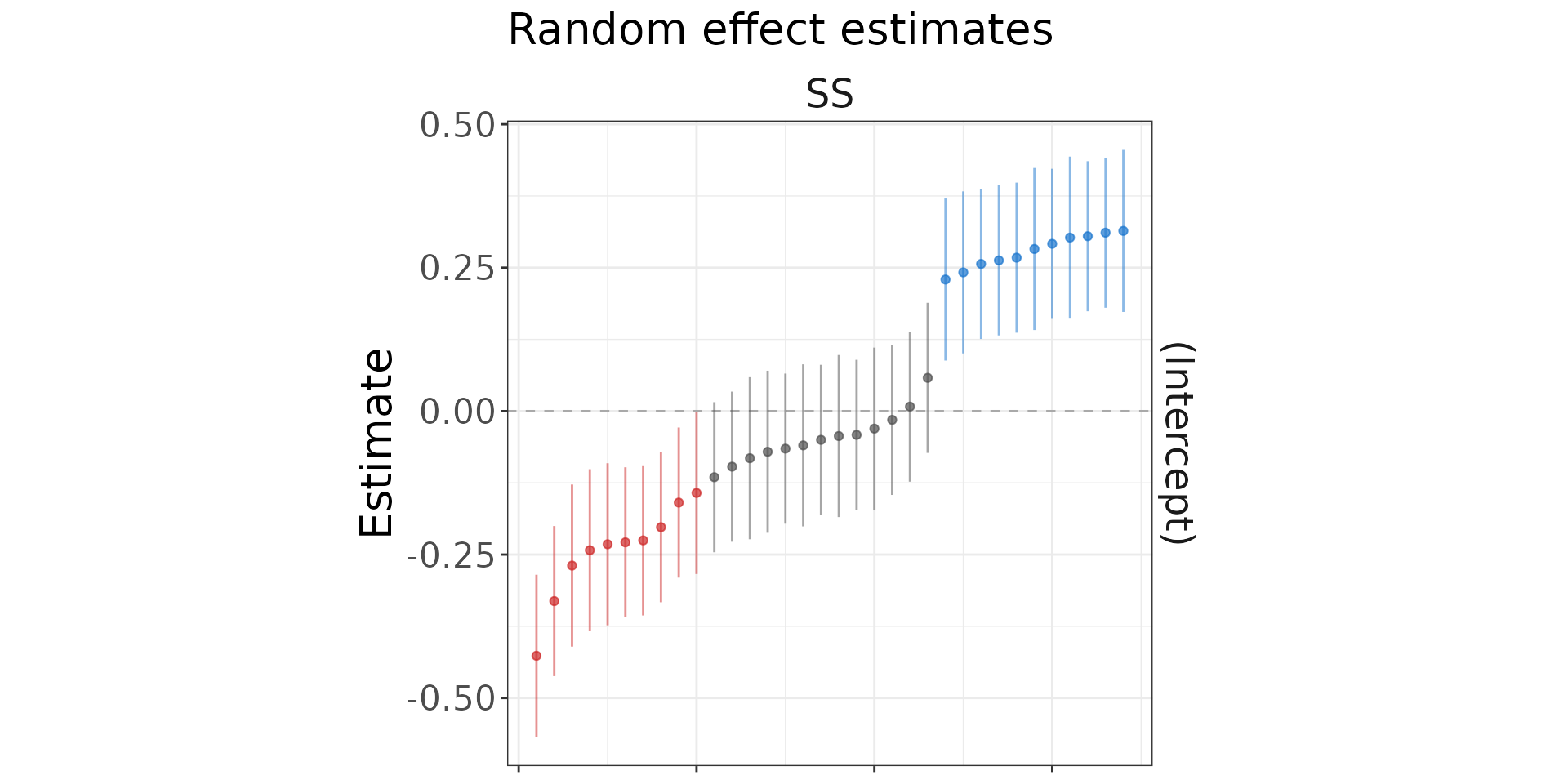
hib_ta_mod$plot("random-effects")
#> Warning: `label` cannot be a <ggplot2::element_blank> object.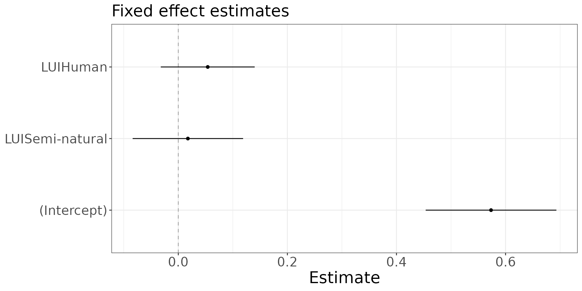
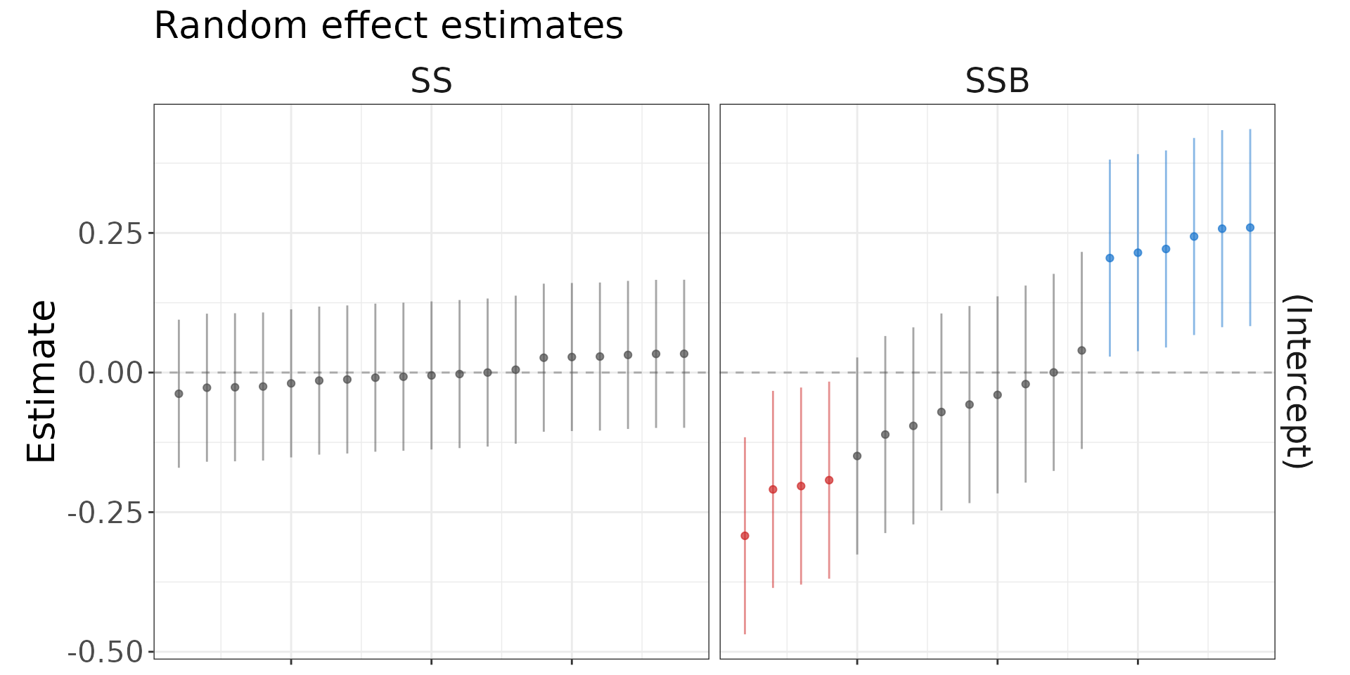
# Check the bray-curtis model
hib_bc_mod$plot()
#> Warning: `label` cannot be a <ggplot2::element_blank> object.

hib_bc_mod$plot("random-effects")
#> Warning: `label` cannot be a <ggplot2::element_blank> object.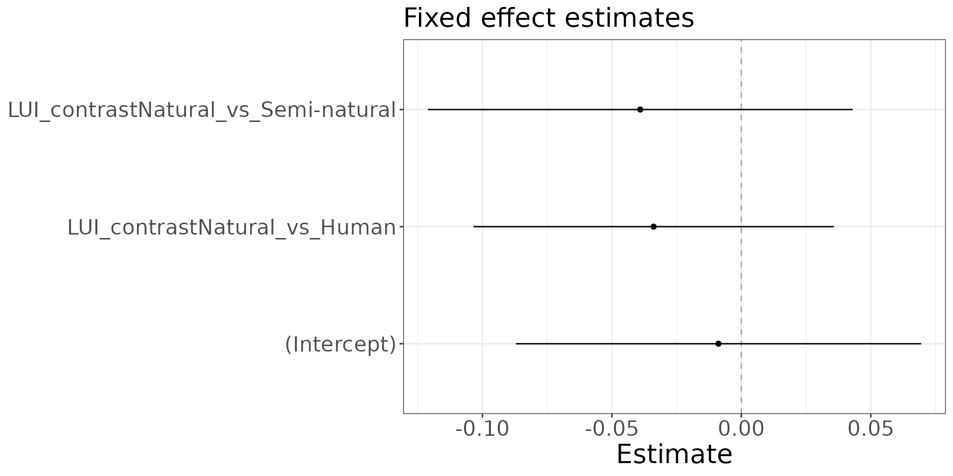
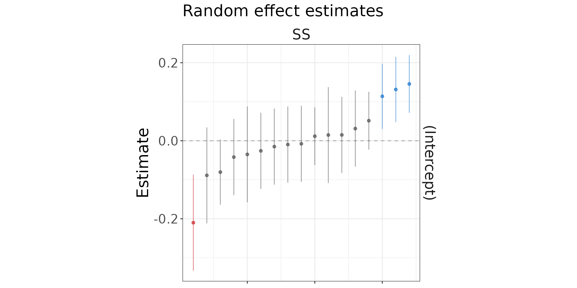
6. Cross-validate the fitted model, using both Random, and geographically blocked folds.
# Cross-validate model, include a back-transformation to obtain predictions/errors
# on the scale of Rescaled_total_abundance
# We also include evaluations when considering the exclusion of random effects,
# and when incorporating the SS random effect into cross-validation predictions.
hib_cv <- hib_cv_model(hib_ta_mod,
                       hib_db,
                       fold_type = c("Random-5", "UN_region"),
                       re_form = list(NA, ~(1|SS)),
                       backtransform = function(x){x^2})
#> Cross-validating supplied lme4 model:
#>  sqrt(Rescaled_total_abundance) ~ LUI + (1 | SS) + (1 | SSB)
#>
#>
#> Running cross-validation using: Random-5
#>
#>     Total number of folds: 5
#>
#>  Progress
#>   |                                                                              |                                                                      |   0%
#> Warning in checkConv(attr(opt, "derivs"), opt$par, ctrl = control$checkConv, :
#> unable to evaluate scaled gradient
#> Warning in checkConv(attr(opt, "derivs"), opt$par, ctrl = control$checkConv, : Model failed to converge: degenerate  Hessian with 1 negative eigenvalues
#>   See ?lme4::convergence and ?lme4::troubleshooting.
#>   |                                                                              |==================                                                    |  25%
#> Warning in checkConv(attr(opt, "derivs"), opt$par, ctrl = control$checkConv, : unable to evaluate scaled gradient
#> Warning in checkConv(attr(opt, "derivs"), opt$par, ctrl = control$checkConv, : Model failed to converge: degenerate  Hessian with 1 negative eigenvalues
#>   See ?lme4::convergence and ?lme4::troubleshooting.
#>   |                                                                              |===================================                                   |  50%  |                                                                              |====================================================                  |  75%
#> Warning in checkConv(attr(opt, "derivs"), opt$par, ctrl = control$checkConv, : unable to evaluate scaled gradient
#> Warning in checkConv(attr(opt, "derivs"), opt$par, ctrl = control$checkConv, : Model failed to converge: degenerate  Hessian with 1 negative eigenvalues
#>   See ?lme4::convergence and ?lme4::troubleshooting.
#>   |                                                                              |======================================================================| 100%
#> Warning: For combination of cross-validation approach ( Random-5 ) and re_form options specified ( NA ), total number of out-of-sample predictions )380) is different to number of in-sample predictions (190).
#> Warning: For combination of cross-validation approach ( Random-5 ) and re_form options specified ( ~(1 | SS) ), total number of out-of-sample predictions )380) is different to number of in-sample predictions (190).
#>
#>
#> Running cross-validation using: UN_region
#>
#>     Total number of folds: 3
#>
#>  Progress
#> Warning in checkConv(attr(opt, "derivs"), opt$par, ctrl = control$checkConv, : unable to evaluate scaled gradient
#> Warning in checkConv(attr(opt, "derivs"), opt$par, ctrl = control$checkConv, : Model failed to converge: degenerate  Hessian with 1 negative eigenvalues
#>   See ?lme4::convergence and ?lme4::troubleshooting.
#>   |                                                                              |                                                                      |   0%
#> Warning in checkConv(attr(opt, "derivs"), opt$par, ctrl = control$checkConv, : unable to evaluate scaled gradient
#> Warning in checkConv(attr(opt, "derivs"), opt$par, ctrl = control$checkConv, : Model failed to converge: degenerate  Hessian with 1 negative eigenvalues
#>   See ?lme4::convergence and ?lme4::troubleshooting.
#>   |                                                                              |===================================                                   |  50%  |                                                                              |======================================================================| 100%
#> Warning: No predictions made for combination of 'UN_region' cross-validation and random-effects structure '~(1 | SS)'.
#>
#> Generating in-sample performance metrics for comparison.
#>
#>
#> Collating cross-validation output ...
#>
#> Initialising HibCV object ...

print(hib_cv)
#> Hibiiscus cross-validated model (lme4)
#> Last updated: 2026-10-30 22:00:02.706793
#>
#> --------------------
#>
#> Summary of cross-validated model
#>
#> Formula:
#> sqrt(Rescaled_total_abundance) ~ LUI + (1 | SS) + (1 | SSB)
#>
#> Performance metrics:
#> CV type   | N folds |   N | Random-effect structure |                 RMSE | Predictive R²
#> ------------------------------------------------------------------------------------------
#> In-sample |       1 | 190 |                      NA | 0.380 (0.356, 0.403) |        -0.059
#> In-sample |       1 | 190 |               ~(1 | SS) | 0.362 (0.337, 0.385) |         0.039
#> Random    |       5 | 190 |                      NA | 0.383 (0.359, 0.407) |        -0.079
#> Random    |       5 | 190 |               ~(1 | SS) | 0.366 (0.339, 0.391) |         0.018
#> UN_region |       3 | 190 |                      NA | 0.388 (0.363, 0.412) |        -0.105
#> UN_region |       3 |   0 |               ~(1 | SS) |                  N/A |           N/A
Note: other cross-validation approaches include; “Random-2”, “Random-3”, “Random-5”, “Random-10”, “Source_ID”, “SS”, “Country”, “UN_subregion”, “UN_region”, “Biome”, “Realm” and “Custom”. When using “Custom”, any grouping variable can be specified, provided it is present in the site data.
# Create a plot showing how the sites are allocated to different cross-validation folds.
hib_cv$plot("map-sites")
#> Warning: `label` cannot be a <ggplot2::element_blank> object.
#> `label` cannot be a <ggplot2::element_blank> object.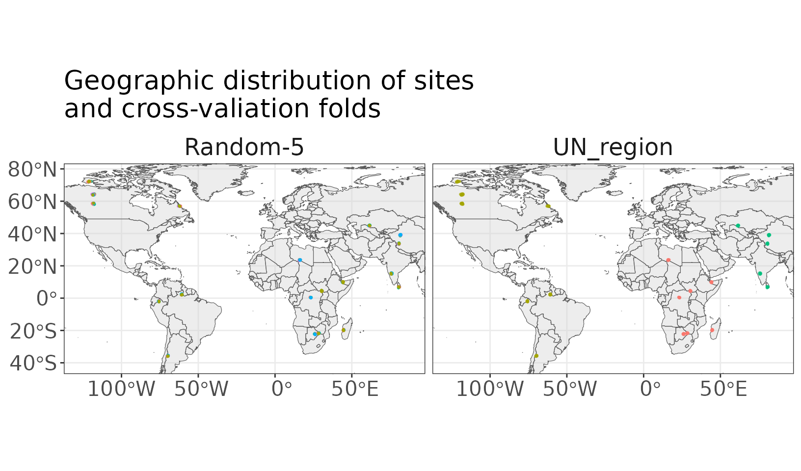
# A figure showing variation in fixed-effects coefficients over cross-validation folds,
# as compared to the coefficients estimated using the complete dataset.
hib_cv$plot("coefficients")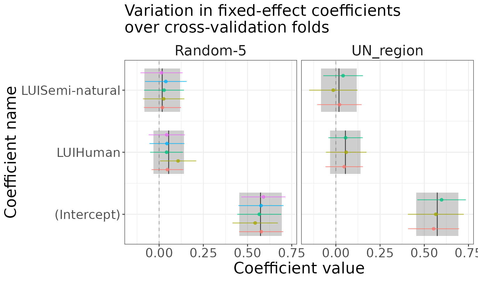
# A simple plot of some key model performance metrics, as estimated via cross-validation.
hib_cv$plot("metrics",
c("corsq", "mae", "rmse", "rsq"))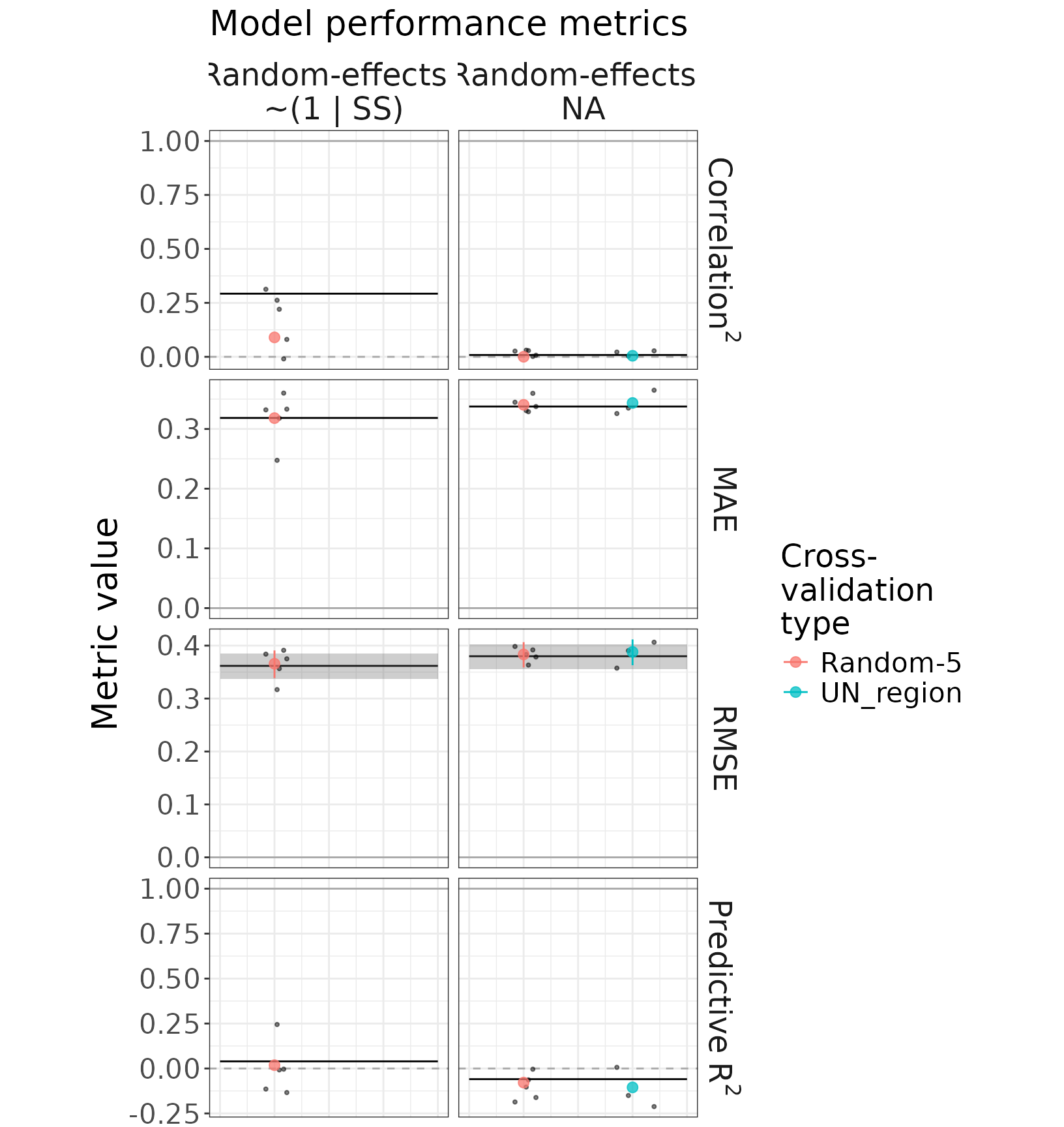 Note: In the above figures displaying coefficients and predictive
performance, the black line and grey shading indicate the values and
confidence intervals, respectively, estimated based on a model fitted to
the complete dataset (In-sample).
7. Model projection
# Generate a simple df of example land-uses for projection.
proj_df <- expand.grid(x = 1:10,
                       y = 1:10) |>
  as.data.frame() |>
  dplyr::mutate(Forest_cover = runif(dplyr::n()),
                LUI = dplyr::case_when(Forest_cover <= 0.3 ~ "Human",
                                              Forest_cover > 0.3 & Forest_cover <= 0.7 ~ "Semi-natural",
                                              Forest_cover > 0.7 ~ "Natural",
                                              T ~ NA))
# Project the fitted model using the example land-use data, including bootstrap
# estimates of uncertainty and an estimate for the area of applicability (AOA).
hib_proj <- hib_project_model(hib_ta_mod,
                              proj_df,
                              backtransform = function(x){x^2},
                              lme4_specs = list(bootstrap = T, n_boot = 50),
                              calc_aoa = T,
                              cv_obj = hib_cv)
#>
#> Estimating Area-of-Applicability...
#> Loading required package: ggplot2
#> Loading required package: lattice
#> Warning in randomForest.default(x, y, mtry = param$mtry, ...): invalid mtry:
#> reset to within valid range
#> Warning in randomForest.default(x, y, mtry = param$mtry, ...): invalid mtry:
#> reset to within valid range
#> Warning in randomForest.default(x, y, mtry = param$mtry, ...): invalid mtry:
#> reset to within valid range
#> Warning in randomForest.default(x, y, mtry = param$mtry, ...): invalid mtry:
#> reset to within valid range
#> Warning in randomForest.default(x, y, mtry = param$mtry, ...): invalid mtry:
#> reset to within valid range
#> Warning in randomForest.default(x, y, mtry = param$mtry, ...): invalid mtry:
#> reset to within valid range
#> Warning in randomForest.default(x, y, mtry = param$mtry, ...): invalid mtry:
#> reset to within valid range
#> Warning in randomForest.default(x, y, mtry = param$mtry, ...): invalid mtry:
#> reset to within valid range
#> Warning in randomForest.default(x, y, mtry = param$mtry, ...): invalid mtry:
#> reset to within valid range
#> Warning in randomForest.default(x, y, mtry = param$mtry, ...): invalid mtry:
#> reset to within valid range
#> Warning in randomForest.default(x, y, mtry = param$mtry, ...): invalid mtry:
#> reset to within valid range
#> note: variables were not weighted either because no weights or model were given,
#>     no variable importance could be retrieved from the given model, or the model has a single feature.
#>     Check caret::varImp(model)
#> CAST warning: predictors contain categorical variables. The integration is currently still under development. Please check results carefully!
#>
#> Warning: rescale_specs missing, using default values:
#>   rescale = FALSE,
#>   baseline_covar = NULL,
#>   baseline_re_form = NA ...
#>
#> lme4 model detected! Projection in progress...
#>
#> Warning: re_form missing from lme4_specs, using default value of NA ...
#>
#> Warning: calc_se missing from lme4_specs, using default value of TRUE ...
#>
#> Warning: conf_level missing from lme4_specs, using default value of 0.95 ...
#>
#> Preparing input data for projection...
#>
#> Projecting model...
#>
#> Generating bootstrapped prediciton intervals using 50 bootstrap samples...
#> ================================================================================
#>
#> Calculating standard error of model predictions...
#> Warning: The training data could not be extracted reliably from the model object. Column types, factor levels, or values may have been coerced or altered. It is safer to use `set_modeldata(model, data)` to attach the training data explicitly. Original warning from `insight::get_data()`: Could not recover model data from environment. Please make sure your
#>   data is available in your workspace.
#>   Trying to retrieve data from the model frame now. This warning appears once per session.
#>
#> Initialising HibProjection object ...
Note: In the above, although we have included a calculation of the AOA (calc_aoa = T), all locations within the projection data have LUI values that are within the set of values used to fit the model. There are therefore no locations outside the AOA in this example.
# Visualise our projection.
hib_proj$plot(response_var = "prediction_mean")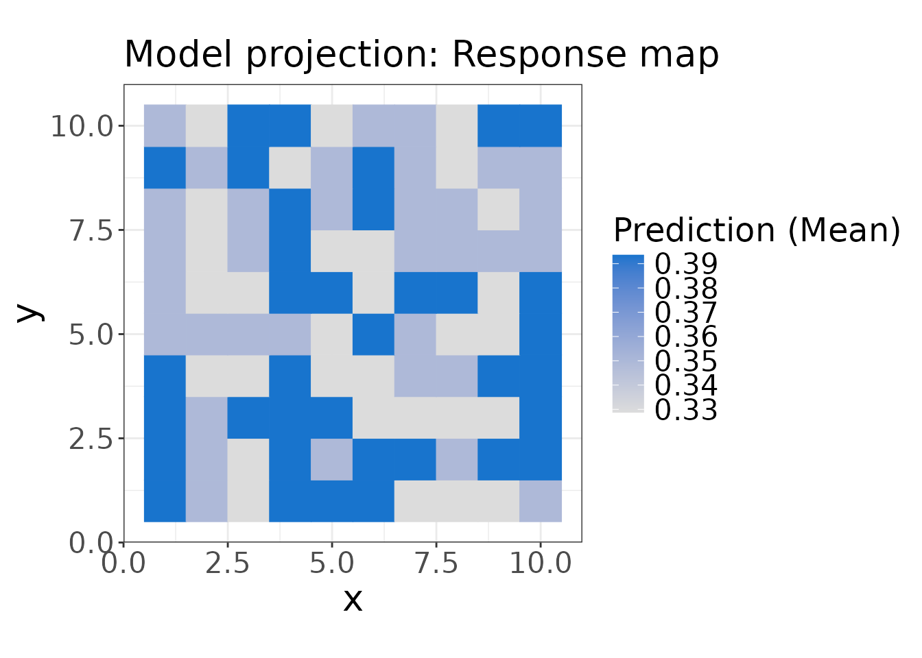
# A figure incorporating both projected values and their uncertainty.
hib_proj$plot("bivariate-map",
              response_var = "prediction_mean",
              uncertainty_var = "prediction_se")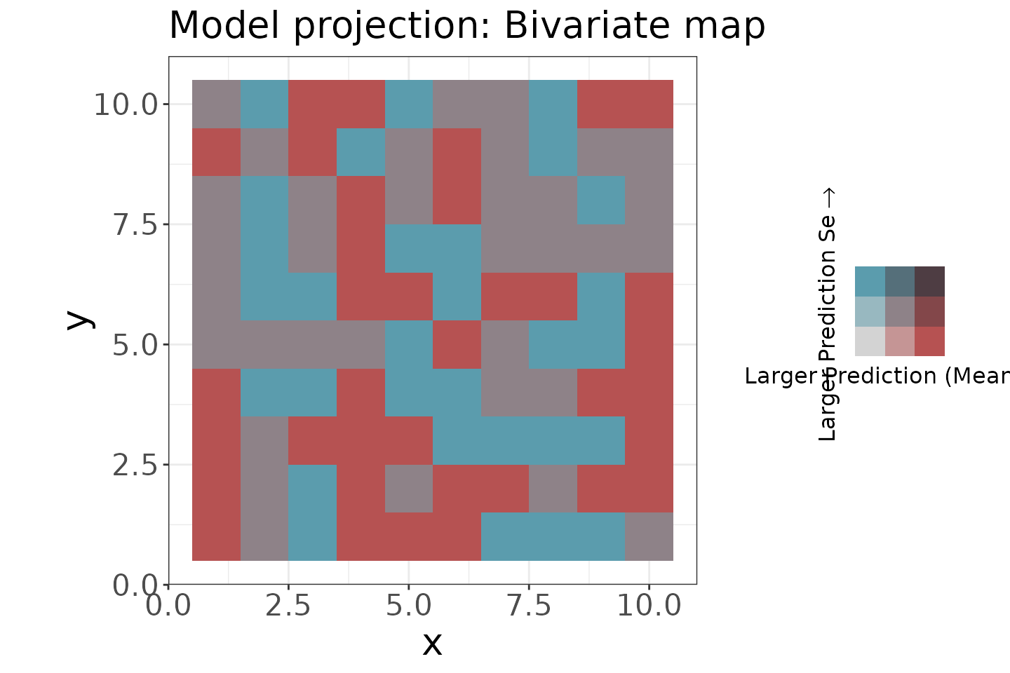
# Check the distribution of projected values.
hib_proj$plot("response-distr", response_var = "prediction_mean")
#> `stat_bin()` using `bins = 30`. Pick better value `binwidth`.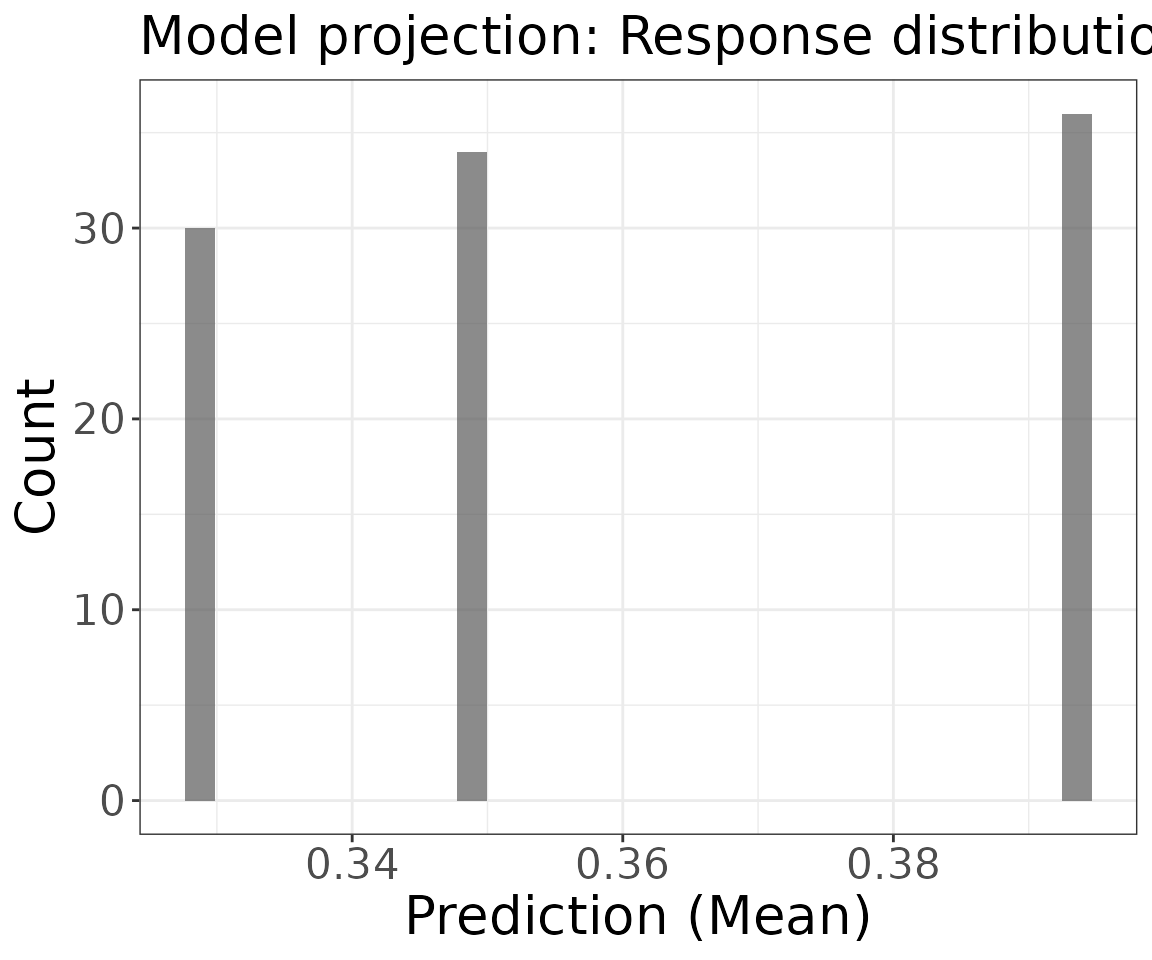
8. Data-integration example
Combine two datasets and fit a mixed-effects model with weights.
# Load our simulated data - and assign the dataset an identifying name.
hib_db2 <- hib_create_db(path_species = system.file("extdata", "dummy_species_rc_2.rds",
                                                   package = "hibiiscus", mustWork = TRUE),
                       dataset_name = "Dummy data 2")
#>
#> Initialising HibDatabase using Dummy data 2 data ...
#>
#> Generating sites dataframe...
#>

# View a summary of the hib database object
print(hib_db2)
#> Hibiiscus database (including dataset/s: Dummy data 2)
#> Last updated: 2026-10-30 22:00:08.749419
#>   Number of sites:               150
#>   Number of species:             939
#>   Number of taxa (orig. names):  939
#>   Land use (class x intensity):  4 x 3
#>   LU/I legend sourced from:      Original LU/I legend.
#>   Database updates:              NA
#>
#>   Effort-correction applied:     FALSE
#>   Filtering conducted:           NA
#>   Data columns added:            NA
#>
#>   Within-site diversity metrics calculated:   NA
#>   Between-site diversity metrics calculated:  NA
#>   Site-site contrast metrics calculated:      NA

# dummy_data_2 <- create_dummy_data("species", n_studies = 15)
# hib_db2$plot()

# Make alt_lu_leg using SSBS, Predominant_land_use - re-align to c("Natural", "Semi-natural", "Human")
alt_lu_df2 <- hib_db2$sites[,c("SSBS", "Predominant_land_use")] |>
  dplyr::mutate(Predominant_land_use = dplyr::case_when(Predominant_land_use == "Primary" ~ "Natural",
                                                        Predominant_land_use == "Secondary" ~ "Semi-natural",
                                                        T ~ "Human"),
                Predominant_land_use = factor(Predominant_land_use,
                                              levels = c("Natural", "Semi-natural", "Human")),
                Use_intensity = "",
                LUI = Predominant_land_use)
# Make an lu legend
alt_lu_leg2 <- hib_create_lu_legend(alt_lu_df2)
#>
#> Initialising HibLULegend from data.frame: alt_lu_df2...
#>
# Set the lu legend on the database
hib_db2 <- hib_set_lu_legend(hib_db2, alt_lu_leg2)
#>
#> Setting land-use legend for HibDatabase...
#>
#> Joining with `by = join_by(SSBS)`
#> Joining with `by = join_by(SSBS)`

# hib_db2$sites$LUI |> unique()

# Effort correction
hib_db2$hib_effort_correction()
#>
#> Correcting biodiversity measurements for sampling effort ...
#>

# Biodiversity metric calculations
hib_db2 <- hib_calc_div_within(hib_db2,
                              c("Total_abundance"))
#>
#> Calculating within-site biodiversity metrics ...
#>
#>     Total abundance ...
#>

hib_ta_mod2 <- hib_fit_lme4(obj = hib_db2,
                            form = sqrt(Rescaled_total_abundance) ~ LUI + (1|SS),
                            REML = F,
                            calc_CIs = "Wald")
#>
#> Collating data for model fitting...
#>
#> Fitting model (this may take some time) ...
#>
#> Collating model details ...
#>
#>     Getting confidence intervals ...
#>
#> Initialising HibModelLME4 object ...

# Modelling
hib_int_mod <- hib_fit_lme4(obj = list(hib_db,
                                       hib_db2),
                            form = sqrt(Rescaled_total_abundance) ~ LUI + (1|SS),
                            REML = F,
                            calc_CIs = "Wald",
                            weight_specs = list(weights = c(0.6, 0.4),
                                                weight_type = "dataset"))
#>
#> Collating data for model fitting...
#>
#> Fitting model (this may take some time) ...
#>
#> Collating model details ...
#>
#>     Getting confidence intervals ...
#>
#> Initialising HibModelLME4 object ...

hib_ta_mod2$dataset_name
#> [1] "Dummy data 2"
hib_ta_mod2$processing_flags
#> $measures_effort_corrected
#> [1] TRUE
#>
#> $abundance_rescaled
#> [1] FALSE
#>
#> $filtering_steps
#> list()
#>
#> $database_updates
#> list()
#>
#> $joined_information
#> list()
#>
#> $lu_legend_source
#> [1] "data.frame ('alt_lu_df2')"
#>
#> $N_spp
#> [1] 939
#>
#> $N_taxa
#> [1] 939
#>
#> $N_sites
#> [1] 150

hib_int_mod$dataset_name
#> [[1]]
#> [1] "Dummy data"
#>
#> [[2]]
#> [1] "Dummy data 2"
hib_int_mod$processing_flags
#> [[1]]
#> [[1]]$measures_effort_corrected
#> [1] TRUE
#>
#> [[1]]$abundance_rescaled
#> [1] FALSE
#>
#> [[1]]$filtering_steps
#> [[1]]$filtering_steps[[1]]
#> [1] "1: UN_region != 'Oceania'"
#>
#>
#> [[1]]$database_updates
#> list()
#>
#> [[1]]$joined_information
#> list()
#>
#> [[1]]$lu_legend_source
#> [1] "data.frame ('alt_lu_df')"
#>
#> [[1]]$N_spp
#> [1] 868
#>
#> [[1]]$N_taxa
#> [1] 868
#>
#> [[1]]$N_sites
#> [1] 190
#>
#>
#> [[2]]
#> [[2]]$measures_effort_corrected
#> [1] TRUE
#>
#> [[2]]$abundance_rescaled
#> [1] FALSE
#>
#> [[2]]$filtering_steps
#> list()
#>
#> [[2]]$database_updates
#> list()
#>
#> [[2]]$joined_information
#> list()
#>
#> [[2]]$lu_legend_source
#> [1] "data.frame ('alt_lu_df2')"
#>
#> [[2]]$N_spp
#> [1] 939
#>
#> [[2]]$N_taxa
#> [1] 939
#>
#> [[2]]$N_sites
#> [1] 150

is.list(hib_ta_mod2$processing_flags)
#> [1] TRUE
is.list(hib_int_mod$processing_flags)
#> [1] TRUE

names(hib_ta_mod2$processing_flags)
#> [1] "measures_effort_corrected" "abundance_rescaled"
#> [3] "filtering_steps"           "database_updates"
#> [5] "joined_information"        "lu_legend_source"
#> [7] "N_spp"                     "N_taxa"
#> [9] "N_sites"
names(hib_int_mod$processing_flags)
#> NULL

is.null(names(hib_ta_mod2$processing_flags))
#> [1] FALSE
is.null(names(hib_int_mod$processing_flags))
#> [1] TRUE
# Check the abundance model
hib_int_mod$plot()
#> Warning: `label` cannot be a <ggplot2::element_blank> object.

hib_int_mod$plot("random-effects")
#> Warning: `label` cannot be a <ggplot2::element_blank> object.