1. Generating GLOBIOM scenario plots • globiomvis

Introduction

To quickly inspect GLOBIOM runs it is often useful to compare historical trends of key variables with model projections. The package includes several functions to support this task. trend_plot_all() produces a PDF file with plots for key combinations of variables, items and units across all GLOBIOM regions for which data is created.trend_plot() generates individual plots for selected variables, items, units and regions. Before these functions can be used historical data and globiom output needs to be loaded first.

Loading and preparing data

Start by loading the required packages.

library(gdxrrw)
library(dplyr)
library(tidyr)
library(purrr)
library(ggplot2)
library(globiomvis)

This will work if you have followed the installation instructions. Provided that you have set the R_GAMS_SYSDIR environment variable, *`gdxrrw will load the GAMS GDX libraries when subsequently issuing:

igdx("")

We load a GLOBIOM output file. We use setNames() to add column names. These will be missing if the gams data table (i.e. the Symbol) has ’*‘instead of set names. We also ensure that YEAR is an integer (and not a character) and ITEM_AG, VAR_ID and VAR_UNIT are in capitals, and add a ’source’ column.

globiom_path <- "P:/globiom"
globiom_file <- file.path(globiom_path, "projects/TEMP/globiom_results/MODEL_OUTPUT_AG_SSP2_lookup_q_SDG_10052019.gdx")
symbol <- "OUTPUT_AG"
globiom <- rgdx.param(globiom_file, symbol) %>%
  setNames(c("VAR_ID", "VAR_UNIT", "REGION_AG", "ITEM_AG", "MacroScen", "BioenScen", "IEA_Scen", "YEAR", "OUTPUT_AG")) %>%
  mutate(YEAR = as.integer(as.character(YEAR)),
         ITEM_AG = toupper(as.character(ITEM_AG)),
         VAR_ID = toupper(VAR_ID),
         VAR_UNIT = toupper(VAR_UNIT),
         source = "globiom") %>%
  droplevels

We also load the historical FAOSTAT data, aggregated to GLOBIOM nomenclature and make some adjustments in the same way as we did for the globiom data file.

hist <- rgdx.param(file.path(globiom_path, "projects/TEMP/globiom_results/OUTPUT_FAO_REGION_since1961_ag_NSUST.gdx"), "OUTPUT_AG") %>%
  mutate(YEAR = as.integer(as.character(YEAR)),
         ITEM_AG = toupper(as.character(ITEM_AG)),
         VAR_ID = toupper(VAR_ID),
         VAR_UNIT = toupper(VAR_UNIT),
         source = "historical") %>%
  droplevels

Create a PDF with plots for key variable, item and unit combinations

Main combinations of globiom variables (VAR_ID), items (ITEM_AG) and units (VAR_UNIT) are stored in main_output_comb. The function trend_plot_all() creates a PDF file with plots for all of these output combinations (and are present in the GLOBIOM output file). In the example below the PDF file with the name globiom_trend_plots_YYYY-MM_DD.pdf is saved to a temporary directory. You may want to change the path parameter to a more permanent location. Note that it might take a bit of time as more than 200 plots are generated.

# Show main combinations of globiom variables
data("main_output_comb", package="globiomvis")
print(main_output_comb)

trend_plot_all(df_gl = globiom, df_hs = hist, path = tempdir())

Create plots for your own selection of GLOBIOM output

It is also possible to create a PDF with a subset of combinations. The function all_output_comb() creates a data frame with all VAR_ID, ITEM_AG and VAR_UNIT combinations in a globiom output file. This file can be used as a basis to filter out relevant output combinations. Alternatively, one can use main_output_comb as a basis or create a new data frame with output combinations.

comb_sel <- all_output_comb(globiom) %>%
  filter(VAR_ID %in% c("AREA", "PROD"), ITEM_AG %in% c("CORN", "CRPLND"), VAR_UNIT %in% c("1000 HA", "1000 T"))

trend_plot_all(df_gl = globiom, df_hs = hist, path = tempdir(), comb = comb_sel, file_name = "globiom_selected")

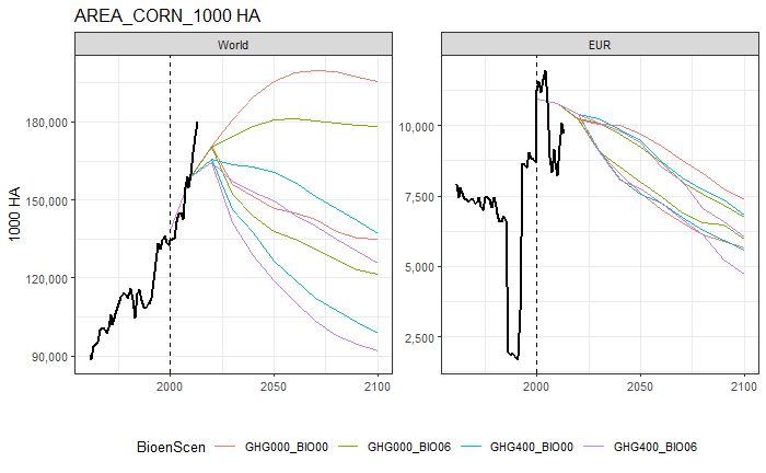
If you want full flexibility to plot the GLOBIOM results, for instance by zooming on a subset of scenarios for a selected number of variables, items and units, it is easier to use the basic function trend_plot(). The following example uses trend_plot() to create a plot for VAR_ID = AREA, ITEM_AG = 1000 HA, VAR_UNIT = 1000 HA, regions: World and EUR and two scenarios: GHG000_BIO00 and GHG000_BIO06. Note that the function gives an error if the combination of variables is not present in the data.

trend_plot(var = "AREA", item = "CORN", unit = "1000 HA", reg = c("World", "EUR"), df_gl = globiom, df_hs = hist)

If you want multiple figures, one has to loop this function over a selection of the data. This requires some additional code and is illustrated below.

# Select scenarios, variables, items and units
var_sel <- c("AREA", "PROD")
item_sel <- c("CORN", "CRPLND")
unit_sel <- c("1000 HA", "1000 T")
reg_sel <- c("World", "EUR")
scen_sel <- c("GHG000_BIO00", "GHG000_BIO06")

# Create data frame with selected GLOBIOM output
globiom_sel <- globiom %>%
  filter(VAR_ID %in% var_sel , ITEM_AG %in% item_sel , VAR_UNIT %in% unit_sel, BioenScen %in% scen_sel)

# Create data frame with unique output combinations in selected globiom output
sel_output_comb <- all_output_comb(globiom_sel)

# Loop over VAR_ID, ITEM_AG and VAR_UNIT
pdf(file = file.path(tempdir(), paste0("globiom_trend_plots_loop_", Sys.Date(), ".pdf")))
purrr::walk(1:nrow(sel_output_comb), function(i){
  trend_plot(var   = sel_output_comb$VAR_ID[i],
             item  = sel_output_comb$ITEM_AG[i],
             unit  = sel_output_comb$VAR_UNIT[i],
             reg   = reg_sel,
             df_gl = globiom_sel,
             df_hs = hist)
})
dev.off()