5  Objective functions

One of the most powerful abilities of mixed or integer linear programming (MILP) compared to other prioritization software approaches is the possibility of readily exchanging objective functions dependending on the question to be answered or the planning objective.In theory many different objective functions could be used in SCP if they can be mathematically formulated (down to complex non-linear optimizations that maximize both area and population abundance of species).

A common distinction among objective functions is whether they make use of a “budget” (e.g. how much total area at most) and/or “targets” (how much of a feature). There are even some objective functions that require neither. Furthermore objective functions differ in their ability of how benefits are accumalted, such as for instance that every little improvement towards a target counts (linear) or whether the whole target needs to be achieved (approaching a step function).

The most classical objective functions are the minimum set and the maximum coverage function (Cabeza & Moilanen (2001)), both of which we introduce below. However other objective functions are possible as well and the prioritizr package focusses primarily on a range of common objective functions used in the context of area-based conservation planning. In the examples below we focus on implementation and less on a detailed mathematical description of the objective functions. Here please have a look at the prioritizr help files.

For a good and more recent literature overview and comparison of different objective functions, we recommend the following reading materials (Cabeza & Moilanen 2001; Arponen et al. 2005; Beyer et al. 2016; Alagador & Cerdeira 2020)

About the use of targets

Most - but not all - objective functions require the use of targets in some way. Although for example the maximum utility objective function works without targets, it is usually not recommend owing to larger assumptions on how benefits for features accumulate (see also Section 3.8).

5.1 Target-based objective functions

5.1.1 Minimum set

The minimum set objective function is the most commonly applied on and also the one exclusively supported by the popular Marxan software (see Ball et al. (2009), and https://marxansolutions.org/). It does not use budgets, but rather tries to identify the minimum amount of area that would satisfy all targets.

Note

If the feature targets are too ambitious it might not be feasible to find a solution for a problem specified with this objective function. Similarly if all targets are set to 100% it naturally will require all PU where the features are present.

# Define a minimum set problem and solve
s1 <- problem(PU, spp) |>                     
  add_min_set_objective() |>
  add_relative_targets(targets = 0.3) |>     
  add_binary_decisions() |>                  
  add_default_solver() |> 
  solve()
1
Defined here. If no targets are specified, an error will be raised.

A minimum set objective function

5.1.2 Maximum coverage objective

The next very commonly used objective function is the maximum coverage objective. This objective seeks to reach as many targets as possible without exceeding a set budget and meeting any cost. Here it differs from the minimum set problem as it is also constrained by a budget and not only by the targets ( Cabeza & Moilanen (2001) ).

Maximum coverage solutions often benefit from additional constraints or penalties that help to prevent the occurrence of many small fragmented patches.

Note

In prioritizr this objective function is (confusingly) called “add_max_features_objective()”

# A dummy 30% of PU area budget
budget.area <- round(0.3 * terra::global(PU,"sum",na.rm=T)[,1])

s2 <- problem(PU, spp) |>    
  add_max_features_objective(budget = budget.area)  |>
  add_relative_targets(targets = 0.3)  |>
  add_binary_decisions() |>                                        
  add_default_solver() |> 
  solve()
1
Sets the objective using the budget specified above.
2
Dummy targets to secure at least 30% of each feature distribution while staying within the budget. Given the large area budget, this should be easy to solve.

Maximum coverage objective function

5.1.3 Minimum shortfall

Closely related to the maximum coverage objective function is the (new’ish) minimum shortfall objective. This objective function tries to, instead of maximizing the coverage of features targets, minimizes the difference between the target and amount in the solution ( Arponen et al. (2005)). Because of the way it is formulated, it is particular useful for conservation problems that have proportional allocation and intend to have benefits increase linearly (Jung et al. (2021)).

In the example below we try to emulate that by trying to secure not only the distribution of tree species but also a reasonable amount of greenness (NDVI). For the latter we set the target to 100%, thus aiming to secure as much as we can together with the other targets.

Sensu Jung et al. (2021) it can also be beneficial here to specify weights particular for features that are numerically underrepresented (if the goal is equivalent representation in the solution).

# A dummy 30% of PU area budget
budget.area <- round(0.3 * terra::global(PU,"sum",na.rm=T)[,1])

# Define targets
tr <- matrix(nrow = terra::nlyr(spp)+1)
tr[,1] <- .3
tr[nrow(tr),] <- 1

s3 <- problem(PU, c(spp, ndvi)) |>
  add_min_shortfall_objective(budget = budget.area)  |>
  add_relative_targets(targets = tr)  |>
  add_binary_decisions() |>                                        
  add_default_solver() |> 
  solve()
1
We set the manual relative targets here equal to the number of features in the problem. Note the +1 to account for the added NDVI.
2
Target for the last feature (NDVI) set to 100%, thus will never be reached.
3
Adding both species and NDVI layer here as a proxy of vegetation greenness
4
The minimum shortfall objective with the 30% budget.
5
Adding the manually defined targets by feature from above here.

A minimum shortfall solution with vegetation amount

5.1.4 Minimum shortfall (largest)

This objective function is very similar to the one above, with the notable difference being mathematically that it minimizes the largest target shortfall, instead of the total (weighted sum) of all target shortfalls.

# Budgets and targets as for minimum shortfall objective!

s4 <- problem(PU, c(spp, ndvi)) |>                                  
  add_min_largest_shortfall_objective(budget = budget.area)  |>       
  add_relative_targets(targets = tr)  |>                              
  add_binary_decisions() |>                                        
  add_default_solver() |> 
  solve()

Minimizing the largest shortfall instead of the sum across features

5.1.5 Other objective functions (phylogenetic)

There are two more objective functions supported by the package that are specifically customized towards phylogenetic data and inter-species relationships. Since those are rather specific, we do not cover them specifically in this tutorial. You can read more about them here and here if of interest.

5.2 Non-target based objective functions

5.2.1 Maximum utility

The maximum utility objective function is one of the objective functions that does not require any targets. It essentially maximizes utility (or feature abundance) within a given budget across features.

Warning

Because of the way it is set up mathematically it can be biased towards areas where particular common species occur as it does maximize across all features equally. The use of weights, costs or penalities is thus highly recommended.

# A dummy 30% of PU area budget
budget.area <- round(0.3 * terra::global(PU,"sum",na.rm=T)[,1])

s5 <- problem(PU, spp) |>    
  add_max_utility_objective(budget = budget.area)  |>
  add_binary_decisions() |>                  
  add_default_solver() |> 
  solve()
1
Note the difference in name (utility vs coverage). The maximum utility objective does not require targets, only a specified budget.

Maximum utility objective function solution

5.2.2 Maximum cover

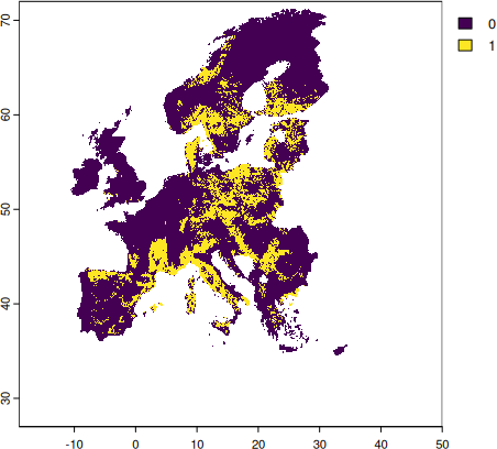
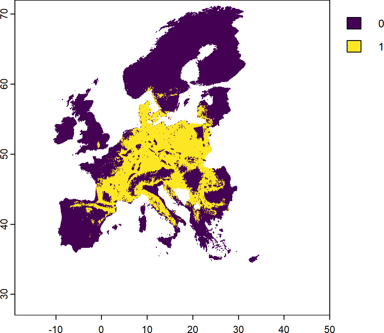
Another objective function without any targets is the maximum coverage objective function. This searches for solutions that represent at least one instance of as many features as possible within a given budget.

Since it does not aim to secure as much as possible, only at least a single PU containing the features, this objective function is usually used for SCP problems where features are highly compartmentalized and a large number of categorical and/or continuous layers is used.

Note

Not to be confused with the “add_max_features_objective()” objective function!

# We subset the data to the alps here for demonstration purposes
alps <- sf::st_read('data/AlpineConvention.shp') |>
  sf::st_transform(crs = sf::st_crs(4326))

PU_alps <- PU |> terra::crop(alps) |> terra::mask(alps)
PA_alps <- PA |> terra::crop(alps) |> terra::mask(alps)
stPA_alps <- stPA |> terra::crop(alps) |> terra::mask(alps)
spp_alps <- spp |> terra::crop(alps) |> terra::mask(alps)
spp.rcp85_alps <- spp.rcp85 |> terra::crop(alps) |> terra::mask(alps)

# We will modify some features for the use of this objective function.
# Specifically we create reclassified versions of features and protected areas
spp1 <- c(PA_alps * spp_alps); names(spp1) <- paste0("currentpa_",names(spp))
spp2 <- c(stPA_alps * spp_alps); names(spp2) <- paste0("currentstpa_",names(spp))
spp3 <- c(PA_alps * spp.rcp85_alps); names(spp3) <- paste0("futurepa_",names(spp.rcp85))

spp4 <- c(stPA_alps * spp.rcp85_alps); names(spp4) <- paste0("futurestpa_",names(spp.rcp85))

# Combine all
spp_pa <- c(spp1,spp2,spp3,spp4)

# A dummy 30% of PU area budget
budget.area <- round(0.3 * terra::global(PU_alps,"sum",na.rm=T)[,1])

s6 <- problem(PU_alps, spp_pa) |>
  add_max_cover_objective(budget = budget.area)  |>
  add_binary_decisions() |>                  
  add_default_solver() |> 
  solve()
1
Get the share of the current range per species covered by protected areas
2
Get the share of the current range per species covered by strictly protected areas
3
Get the share of the future range per species covered by protected areas
4
Get the share of the future range per species covered by strictly protected areas
5
Define the problem with the features created above (number= 268)
6
Maximum coverage objectives requires only a budget.

Maximum coverage objective function

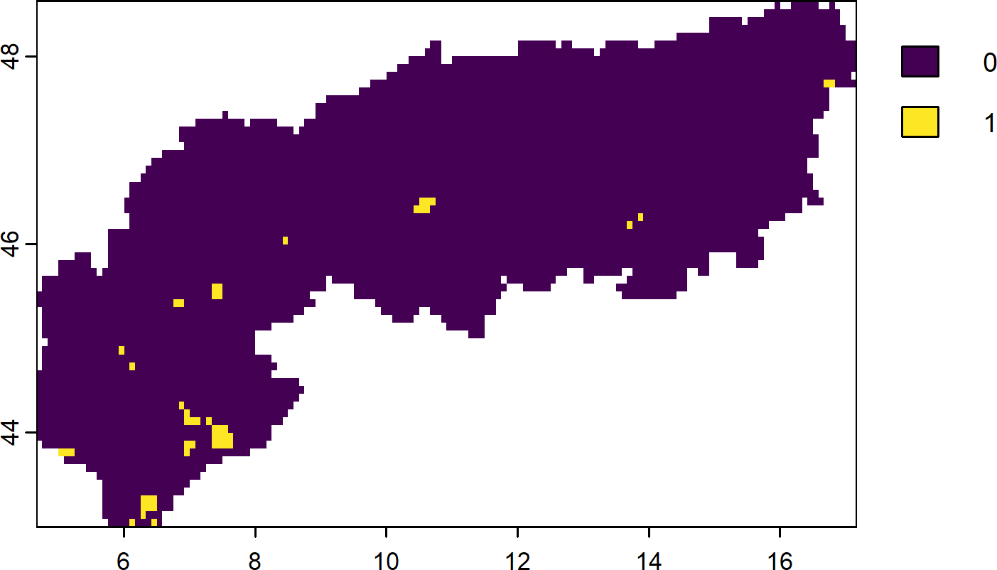
The PU selected in the solution above ensure that each of the 268 features considered (current and future protected species) are covered at least once somewhere in the study region.