2. Economy

2.1. Gross world product (GWP)

Gross world product ($GWP$) in the FeliX model is determined by the total reference economic output ($REO$), further influenced by impacts from climate changes ($Imp\_CC\_on\_GWP$) and biodiversity ($Imp\_Biodiv\_on\_GWP$).

\[GWP(t)=REO(t) \times Imp\_CC\_on\_GWP(t) \times Imp\_Biodiv\_on\_GWP(t)\]

(Eq. 2.1)

$Imp\_CC\_on\_GWP$ is related to the climate change damage (details see the section 2.2 Climate impacts on GWP), and $Imp\_Biodiv\_on\_GWP$ is an endogenous variable related to the mean species abundance ($MSA$) from the biodiversity module (the section 9. Biodiversity). The total $REO$ is the sum of the $REO$ generated by the labor force by skill ($REO_{skill}$). As mentioned in 1.5 Labor force, skill of labor force is distinguished into skilled and unskilled. $REO_{skill}$ are computed based on a Cobb‑Douglas production function, depending on the technology ($\varphi\_Tech_{skill}$) and capital ($\varphi\_K_{skill}$) allocated to the labor force, and the size of the labor force input.

\[REO_{skill}(t)= REO\_Init_{skill} \times \varphi \_ Tech _ {skill}(t) \times Tech(t) \times \Big( \varphi \_ K _ {skill}(t) \times \frac {K(t)} {K\_Init} \Big) ^ {CEO_{skill}} \times \sum_{gender}{\sum_{age=“15‒19”}^{“60‒64”}{LF\_Input_{gender,age,skill}(t) ^ {(1-CEO_{skill})} }}\]

(Eq. 2.2)

where $CEO_{skill}$ is the capital elasticity output for skilled and unskilled labor force. $REO\_Init_{skill}$, $\varphi\_Tech_{skill}$, $\varphi\_K_{skill}$, and $CEO_{skill}$ are exogenous parameters determined by model calibration based on historical data of $GWP$ and $GWP\_per\_Cap$ from The World Bank (2020). Technology-related factor productivity ($Tech$) is distinguished into energy technology ($Tech\_Eng$) and all other technology ($Tech\_Oth$). Particularly, $Tech\_Eng$ is endogenously determined by investments in the energy module while $Tech\_Oth$ follows an exogenous trend and data. The labor force input ($LF\_Input_{gender,age,skill}$) is the corresponding labor force multiplied by the labor force participation rates for the respective groups (by gender and age cohort), which is set to be 34‒78% depending on genders and age cohorts following The World Bank (2020).

$GWP\_per\_Cap$ is hence calculated as $GWP$ divided by total population.

\[GWP\_per\_Cap(t)= \frac {GWP(t)} {\sum_{gender}{\sum_{age}{Pop_{gender,age}(t)}}}\]

(Eq. 2.3)

2.2. Climate change impacts on GWP

Impacts of climate change on economy ($Imp\_CC\_on\_GWP$) is reflected in the economic loss due to climate damage, which is defined by a fraction of GWP.

\[Imp\_CC\_on\_GWP(t)= 1-D(t), \ where \ D(t) = \begin{cases} 0 &\text{if $S\_D = 0$} \\ D\_N(t) &\text{if $S\_D = 1$} \\ D\_DS(t) &\text{if $S\_D = 2$} \\ D\_B1(t) &\text{if $S\_D = 3$} \\ D\_B2(t) &\text{if $S\_D = 4$} \\ D\_L(t) &\text{if $S\_D = 5$} \\ \end{cases}\]

(Eq. 2.4)

In FeliX, an optional structure that enables using the damage functions obtained from previous studies (Burke et al., 2015; Dietz and Stern, 2015; Kalkuhl and Wenz, 2020; Nordhaus, 2017; Weitzman, 2012), or a custom function defined in a flexible logistic form (Eq. 2.7). $S\_D$ is a climate damage function switch that allows users to switch between the options.

$D\_N(t)$ is the damage function used by Nordhaus (2017).

\[D\_N(t)= 1-\frac {1} {1+\alpha T(t)+\beta T(t)^2}\]

(Eq. 2.5)

where $T$ is the global mean temperature change from preindustrial times and the parameters $\alpha$ and $\beta$ are -0.00118 and 0.00278, respectively, yielding the percentage damage.

$D\_DS(t)$ is the function used by Dietz and Stern (2015).

\[D\_DS(t)= 1-\frac {1} { 1 + \Big( \frac {T(t)} {\delta _1} \Big) ^ {\varepsilon _1} + \Big( \frac {T(t)} {\delta _2} \Big) ^ {\varepsilon _2} }\]

(Eq. 2.6)

where the parameters $\delta_1$, $\delta_2$, $\varepsilon_1$ and $\varepsilon_2$ are 12.2, 4.0, 2.0 and 7.02, respectively.

$D\_B1$ and $D\_B2$ are short-term pooled and long-term differentiated damage estimates of Burke et al. (2015), and they are defined in a lookup form digitalized from the figures in their paper. Table 2.1 lists those point estimates used in the model.

Table 2.1. Damage estimates of Burke et al. (2015) for short-term pooled (D_B1) and long-term differentiated (D_B2) responses.

T ($^\circ C$)	$D\_B1$ (%)	$D\_B2$ (%)
1.0	1.0	6.3
2.0	13.0	35.0
3.0	19.0	55.0
4.0	20.5	68.7
5.0	21.0	80.0

$D\_L(t)$ is a logistic function that can be used to define custom-shaped damage functions using three parameters $L\_D$ (the saturation level), $k\_D$ (steepness), and $x0\_D$ (the inflection point).

\[D\_L(t)= \frac {L\_D} {1 + e^{-k\_D \times (T(t)-x0\_D)} }\]

(Eq. 2.7)

2.3. Poverty

The global poverty rate ($PR$) is defined as the proportion of the population aged 15+ living below the international extreme poverty line ($PL$, $2.15 per capita per day in 2017 PPP). It is the sum of the poverty rates across the different population groups aged over 15 weighted by their corresponding population shares.

\[PR(t)= \frac {\sum_{gender}{\sum_{age \geq “15‒19”}{PR_{gender,age}(t) \times Pop_{gender,age}(t)}}} {\sum_{gender}{\sum_{age}{PR_{gender,age}(t)}}}\]

(Eq. 2.8)

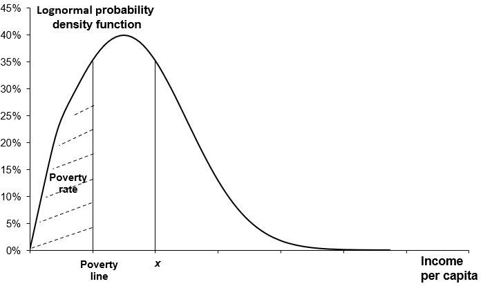
The poverty rate of each population group ($PR_{gender,age}$) is the share of the population living below a specified poverty level $PL$ (Figure 2.1) (Fosu, 2010; Hughes, 2015). When calculating $PR_{gender,age}$, income per capita ($Income\_per\_Cap_{gender,age}$) is assumed to follow a log-normal distribution characterized by the mean ($\mu_{gender,age}$) and standard deviation ($\sigma_{gender,age}$) of the normal distribution function of $\ln(Income\_per\_Cap_{gender,age})$, based on previous research (Fosu, 2010; Lakner et al., 2022; Liu et al., 2023).

\[PR_{gender,age}(t)(Income\_per\_Cap_{gender,age}) \leq PL) = \emptyset \Big( \frac {\ln(PL)- \mu_{gender,age}(t)} {\sigma _{gender,age}(t)} \Big)\]

(Eq. 2.9)


Figure 2.1. The lognormal probability density function of income. The shaded area is equal to the poverty rate.

The standard normal cumulative distribution function can be obtained by looking up the standard normal distribution table.

\[\emptyset \Big( \frac {\ln(Income\_per\_Cap_{gender,age})- \mu_{gender,age}(t)} {\sigma _{gender,age}(t)} \Big) = \int_{-\infty}^ {\frac {\ln(Income\_per\_Cap_{gender,age})- \mu_{gender,age}(t)} {\sigma _{gender,age}(t)} } {\frac {1} {\sqrt{2\pi}} e^{-\frac {(\ln(Income\_per\_Cap_{gender,age}-\mu_{gender,age}(t))^2} {2\sigma ^2 _{gender,age}(t)} } } \,dx\]

(Eq. 2.10)

The probability density function of income is shown in Eq. 2.11 and Figure 2.1 (Fosu, 2010; Mendez Ramos, 2019).

\[f(Income\_per\_Cap,\mu_,\sigma,t) = \frac {1} {\sqrt{2\pi} \sigma _{gender,age}(t)} e^{-\frac {(\ln(Income\_per\_Cap_{gender,age}-\mu_{gender,age}(t))^2} {2\sigma ^2 _{gender,age}(t)} },\ \ln(Income\_per\_Cap) \sim N(\mu_,\sigma)\]

(Eq. 2.11)

To get $PR_{gender,age}$, given the poverty line, only $\mu_{gender,age}$ and $\sigma_{gender,age}$ need to be computed. Eq. 2.12 shows the relationship between $Income\_per\_Cap_{gender,age}$, $\mu_{gender,age}$ and $\sigma_{gender,age}$ (Chotikapanich et al., 1997; Dixon et al., 1987).

\[Income\_per\_Cap_{gender,age}(t) = e^{\mu_{gender,age}(t)} + \frac {\sigma ^2 _{gender,age}(t)} {2}\]

(Eq. 2.12)

where $\mu_{gender,age}$ is a function of $\sigma_{gender,age}$ and $Income\_per\_Cap_{gender,age}$ (Dixon et al., 1987). $\sigma_{gender,age}$ can be expressed as a function of the Gini coefficient.

\[\sigma _{gender,age}(t) = \sqrt{2} \emptyset ^{-1} \Big( \frac {Gini_{gender,age}(t)+1} {2} \Big)\]

(Eq. 2.13)

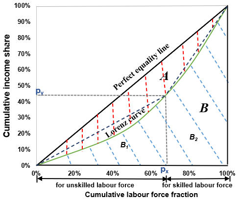
where $\emptyset^{-1}$ is the inverse standard normal cumulative distribution function, and its value can be obtained through the inverse query of the standard normal distribution. To calculate $\mu_{gender,age}$ and $\sigma_{gender,age}$, we thus need to calculate $Gini_{gender,age}$ and $Income\_per\_Cap_{gender,age}$. The Gini coefficient is a numerical value derived from the Lorenz curve (Gastwirth, 1972) as a graphical measure of the income distribution (Figure 2.2). Let $A$ denote the area between the perfect equality line and the Lorenz curve, and $B$ (the sum of $B1$ and $B2$) the area beneath the Lorenz curve (Figure 2.2). $Gini_{gender,age}$ can thus be defined by Eq. 2.14 (Dixon et al., 1987).

\[Gini_{gender,age}(t)= \frac {A_{gender,age}(t)} {A_{gender,age}(t)+B_{gender,age}(t)} = \frac {0.5-B_{gender,age}(t)} {0.5} =1-2B_{gender,age}(t)\]

(Eq. 2.14)


Figure 2.2. Income distribution measured by Lorenz curve. The cumulative labor force fraction at a point on the x-axis is defined as the size of cumulative labor force at this point divided by the size of the total labor force. The x-value of px and a y-value of py mean that the unskilled labor force (the bottom px of the labor force) controls the proportion py of the total income. The Gini coefficient is a numerical value derived from the Lorenz curve to measure income distribution, which is defined as \(A/(A+B)\). Here, \(A\) and \(B\) represent the sizes of the red and blue striped areas. \(B\) is the sum of \(B1\) and \(B2\). The sum of \(A\) and \(B\) is 0.5. The perfect equality line corresponds to a Gini coefficient of 0, indicating that every person has the same income.

Figure 2.2. Income distribution measured by Lorenz curve. The cumulative labor force fraction at a point on the x-axis is defined as the size of cumulative labor force at this point divided by the size of the total labor force. The x-value of px and a y-value of py mean that the unskilled labor force (the bottom px of the labor force) controls the proportion py of the total income. The Gini coefficient is a numerical value derived from the Lorenz curve to measure income distribution, which is defined as $A/(A+B)$. Here, $A$ and $B$ represent the sizes of the red and blue striped areas. $B$ is the sum of $B1$ and $B2$. The sum of $A$ and $B$ is 0.5. The perfect equality line corresponds to a Gini coefficient of 0, indicating that every person has the same income.

By using a triangle and a trapezoid to approximate the areas of $B1$ and $B2$ (Figure 2.2) (Hughes, 2015), $Gini_{gender,age}$ can be reformulated by Eq. 2.15.

\[Gini_{gender,age}(t)= 1- \frac {1} {Tot \_Rel\_Income_{gender,age} \times LF_{gender,age}(t)} \times \Big[ LF_{gender,age,unskilled}(t) \times Rel\_Income_{gender,age,unskilled} + LF_{gender,age,skilled}(t) \times (2 \times Rel\_Income_{gender,age,unskilled}+Rel\_Income_{gender,age,skilled}) \Big]\]

(Eq. 2.15)

where $Tot\_Rel\_Income_{gender,age}$, $Rel\_Income_{gender,age,unskilled}$, and $Rel\_Income_{gender,age,skilled}$ denote the relative income of the total, unskilled, and skilled labor force of the corresponding population group, respectively. $Tot\_Rel\_Income_{gender,age}$ is assumed to be 100. The values of $Rel\_Income_{gender,age,unskilled}$ and $Rel\_Income_{gender,age,skilled}$ are based on relative earnings data for OECD countries (OECD, 2020).

$Income\_per\_Cap_{gender,age}$ is related to the $GWP\_per\_Cap$.

\[Income\_per\_Cap_{gender,age}(t) = GWP\_per\_Cap_{gender,age}(t) \times Real\_Income\_Param_{gender,age}\]

(Eq. 2.16)

where $Real\_Income\_Param_{gender,age}$ is determined by model calibration based on data from the World Bank (2020).

References:

The World Bank (2020). GDP per capita (current US$). https://data.worldbank.org/indicator/NY.GDP.PCAP.CD?name_desc=false.
Nordhaus, W.D. (2017). Revisiting the social cost of carbon. Proceedings of the National Academy of Sciences 114, 1518-1523. https://doi.org/10.1073/pnas.1609244114.
Dietz, S., and Stern, N. (2015). Endogenous growth, convexity of damage and climate risk: How nordhaus’ framework supports deep cuts in carbon emissions. The Economic Journal 125, 574-620. https://doi.org/10.1111/ecoj.12188.
Weitzman, M.L. (2012). Ghg targets as insurance against catastrophic climate damages. Journal of Public Economic Theory 14, 221-244. https://doi.org/10.1111/j.1467-9779.2011.01539.x.
Kalkuhl, M., and Wenz, L. (2020). The impact of climate conditions on economic production. Evidence from a global panel of regions. Journal of Environmental Economics Management 103, 102360. https://doi.org/10.1016/j.jeem.2020.102360.
Burke, M., Hsiang, S.M., and Miguel, E. (2015). Global non-linear effect of temperature on economic production. Nature 527, 235-239. https://doi.org:10.1038/nature15725.
Hughes, B.B. (2015). International futures (ifs) economic model documentation. https://pardee.du.edu/sites/default/files/Economics%20Documentation%20v43%20clean.pdf.
Fosu, A.K. (2010). Inequality, income, and poverty: Comparative global evidence. Social Science Quarterly 91, 1432-1446. 10.1111/j.1540-6237.2010.00739.x.
Lakner, C., Mahler, D.G., Negre, M., et al. (2022). How much does reducing inequality matter for global poverty? The Journal of Economic Inequality, 1-27. https://doi.org/10.1007/s10888-021-09510-w.
Liu, Q., Gao, L., Guo, Z., et al. (2023). Robust strategies to end global poverty and reduce environmental pressures. One Earth 6, 392-408. https://doi.org/10.1016/j.oneear.2023.03.007.
Mendez Ramos, F. (2019). Uncertainty in ex-ante poverty and income distribution: Insights from output growth and natural resource country typologies. World Bank Policy Research Working Paper. 10.1596/1813-9450-8841.
Kakwani, N.C. (1980). Income inequality and poverty (World Bank).
Chotikapanich, D., Valenzuela, R., and Rao, D.P. (1997). Global and regional inequality in the distribution of income: Estimation with limited and incomplete data. Empirical Economics 22, 533-546. 10.1007/BF01205778.
Dixon, P.M., Weiner, J., Mitchell-Olds, T., et al. (1987). Bootstrapping the gini coefficient of inequality. Ecology 68, 1548-1551. 10.2307/1939238.
Gastwirth, J.L. (1972). The estimation of the lorenz curve and gini index. The Review of Economics and Statistics, 306-316. 10.2307/1937992.
OECD (2023). Education and earnings. https://stats.oecd.org/Index.aspx?DataSetCode=EAG_EARNINGS