1) General InSiGHTS functions

This article gives a first tour of the main insights_*() functions. The examples use the small rasters shipped with the package so they can be rendered by pkgdown without external downloads.

Function	Use it when	Main output
`insights_fraction()`	Land-use, habitat, or condition layers are fractions or suitability weights in `[0, 1]`.	A refined suitability or area-of-habitat raster.
`insights_area()`	Land-use or habitat layers are already expressed as area per cell.	A refined raster already in area units.
`insights_discount()`	A habitat class should be discounted by an age or maturity layer.	A maturity-weighted version of the land-use layer.
`insights_summary()`	Refined rasters need to be converted to totals or relative indicators.	A data frame of absolute area, relative change, or symmetric relative change.

library(ibis.insights)
library(terra)
library(stars)

Example inputs

The current range example is a binary range layer. The land-use layers are stored as integer fractions from 0 to 10000, so we divide them by 10000 before passing them to insights_fraction(). The DEM example is already scaled to [0, 1] and is used here as a simple additional suitability mask.

range <- terra::rast(system.file(
  "extdata/example_range.tif",
  package = "ibis.insights",
  mustWork = TRUE
))

grassland <- terra::rast(system.file(
  "extdata/Grassland.tif",
  package = "ibis.insights",
  mustWork = TRUE
)) / 10000

sparse_vegetation <- terra::rast(system.file(
  "extdata/Sparsely.vegetated.areas.tif",
  package = "ibis.insights",
  mustWork = TRUE
)) / 10000

lu_fraction <- c(grassland, sparse_vegetation)
names(lu_fraction) <- c("grassland", "sparse_vegetation")

extra_suitability <- terra::rast(system.file(
  "extdata/DEM.tif",
  package = "ibis.insights",
  mustWork = TRUE
))
names(extra_suitability) <- "extra_suitability"

op <- par(mfrow = c(2, 2), mar = c(2, 2, 3, 4))
plot(range, main = "Range")
plot(lu_fraction[[1]], main = "Grassland fraction")
plot(lu_fraction[[2]], main = "Sparse vegetation fraction")
plot(extra_suitability, main = "Additional suitability mask")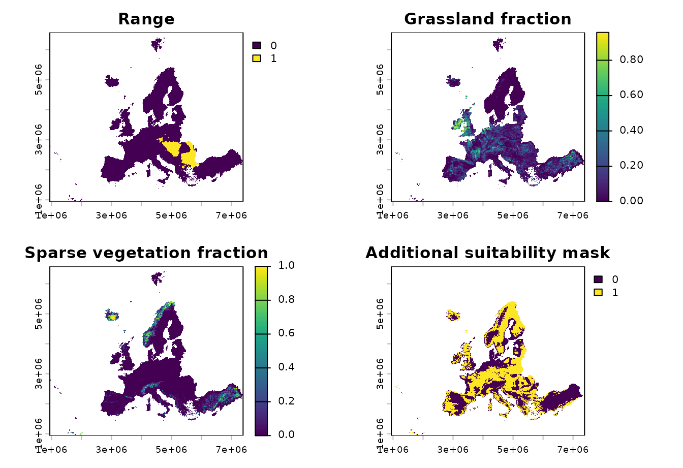

par(op)

Fractional land-use: `insights_fraction()`

Use insights_fraction() when the habitat or land-use input is a fraction, probability, or suitability weight. Multiple land-use layers are summed before they are applied to the range. clamp = TRUE caps the combined suitability at one when several suitable land-use classes overlap.

aoh_fraction <- insights_fraction(
  range = range,
  lu = lu_fraction,
  other = extra_suitability,
  clamp = TRUE
)

plot(aoh_fraction, main = "Fractional InSiGHTS output")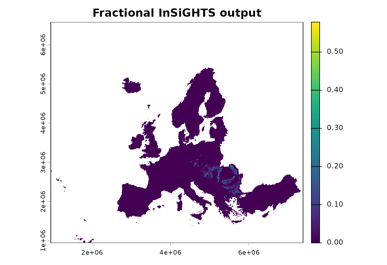

insights_summary() converts this fractional raster to area by multiplying by cell area, because toArea = TRUE by default.

insights_summary(aoh_fraction, relative = FALSE)
#>   time suitability unit
#> 1   NA    23590.72  km2

Areal land-use: `insights_area()`

Use insights_area() when the land-use values are already in area units. In this example we convert the fractional land-use layers to square kilometres per cell with terra::cellSize(). Because the output is already in area units, summarize with toArea = FALSE.

cell_area_km2 <- terra::cellSize(lu_fraction[[1]], unit = "km")
lu_area_km2 <- lu_fraction * cell_area_km2

aoh_area <- insights_area(
  range = range,
  lu = lu_area_km2,
  other = extra_suitability
)

plot(aoh_area, main = "Areal InSiGHTS output (km2 per cell)")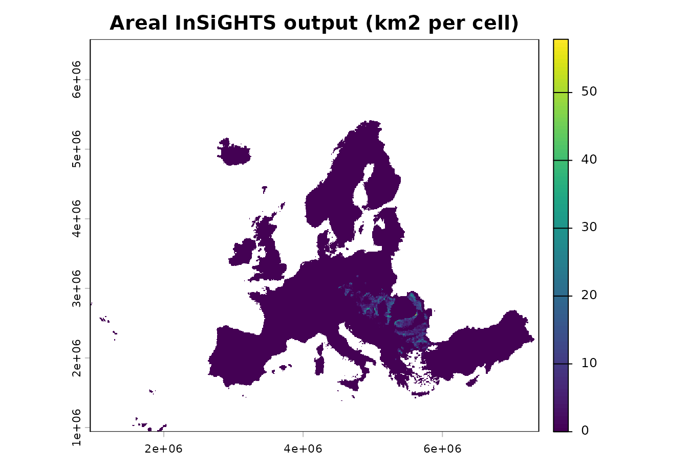

insights_summary(aoh_area, toArea = FALSE, relative = FALSE)
#>   time suitability  unit
#> 1   NA    23590.72 input

Maturity weighting: `insights_discount()`

Use insights_discount() before insights_fraction() or insights_area() when a habitat class should not count at full value immediately after it appears. The example below creates a simple dummy age layer for grassland. Real analyses should use an age or maturity layer for the same habitat class.

grassland_age <- lu_fraction[["grassland"]] * 40
names(grassland_age) <- "grassland_age_years"

invisible(utils::capture.output({
  grassland_discounted <- insights_discount(
    lu = lu_fraction[["grassland"]],
    age = grassland_age,
    target_age = 20,
    target = 0.95
  )
}))
names(grassland_discounted) <- "grassland_discounted"

lu_discounted <- c(grassland_discounted, lu_fraction[["sparse_vegetation"]])
names(lu_discounted) <- c("grassland_discounted", "sparse_vegetation")

aoh_discounted <- insights_fraction(
  range = range,
  lu = lu_discounted,
  other = extra_suitability,
  clamp = TRUE
)

op <- par(mfrow = c(1, 3), mar = c(2, 2, 3, 4))
plot(lu_fraction[["grassland"]], main = "Original grassland")
plot(grassland_age, main = "Dummy age layer")
plot(grassland_discounted, main = "Discounted grassland")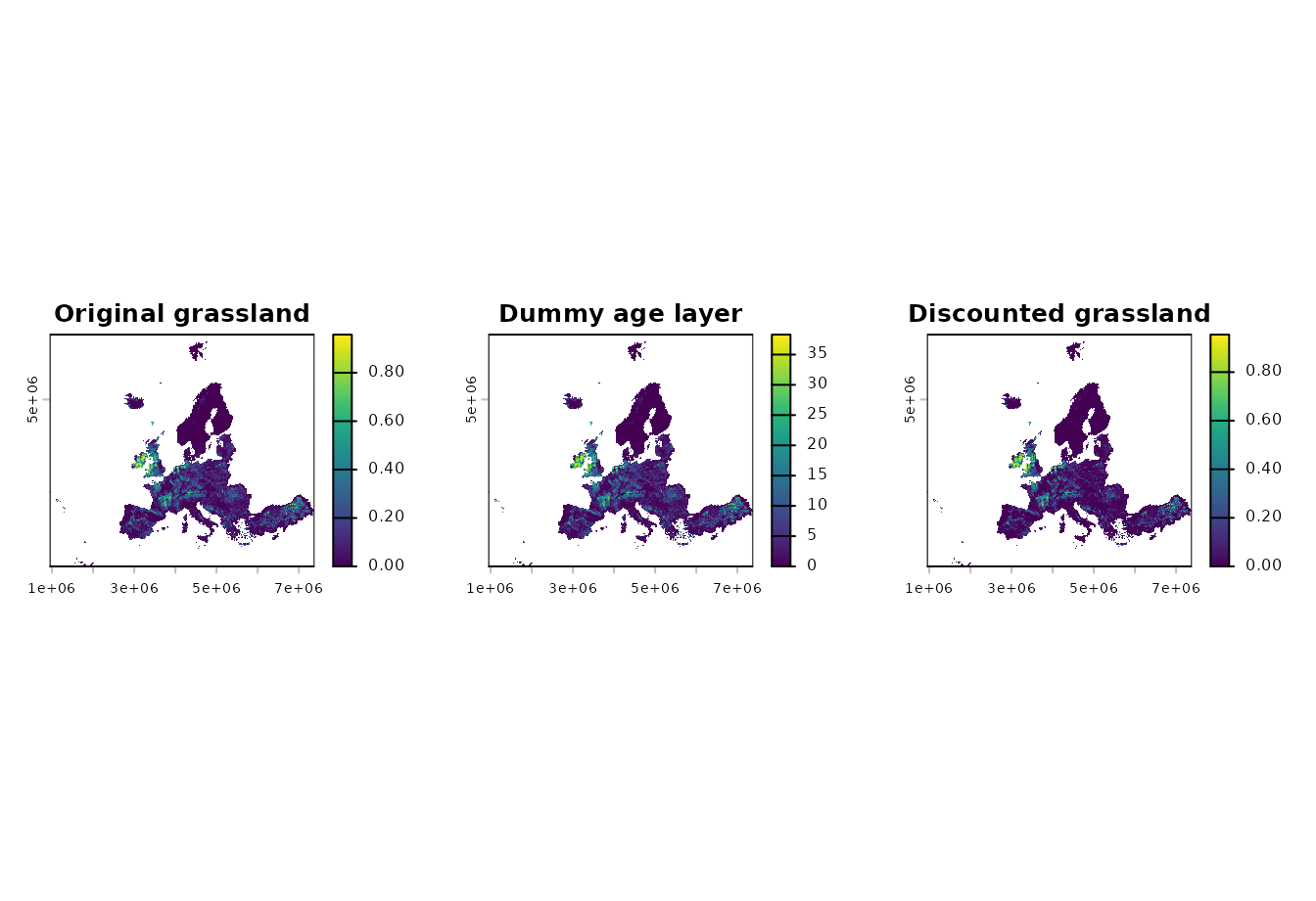

par(op)

op <- par(mfrow = c(1, 2), mar = c(2, 2, 3, 4))
plot(aoh_fraction, main = "Without discount")
plot(aoh_discounted, main = "With grassland discount")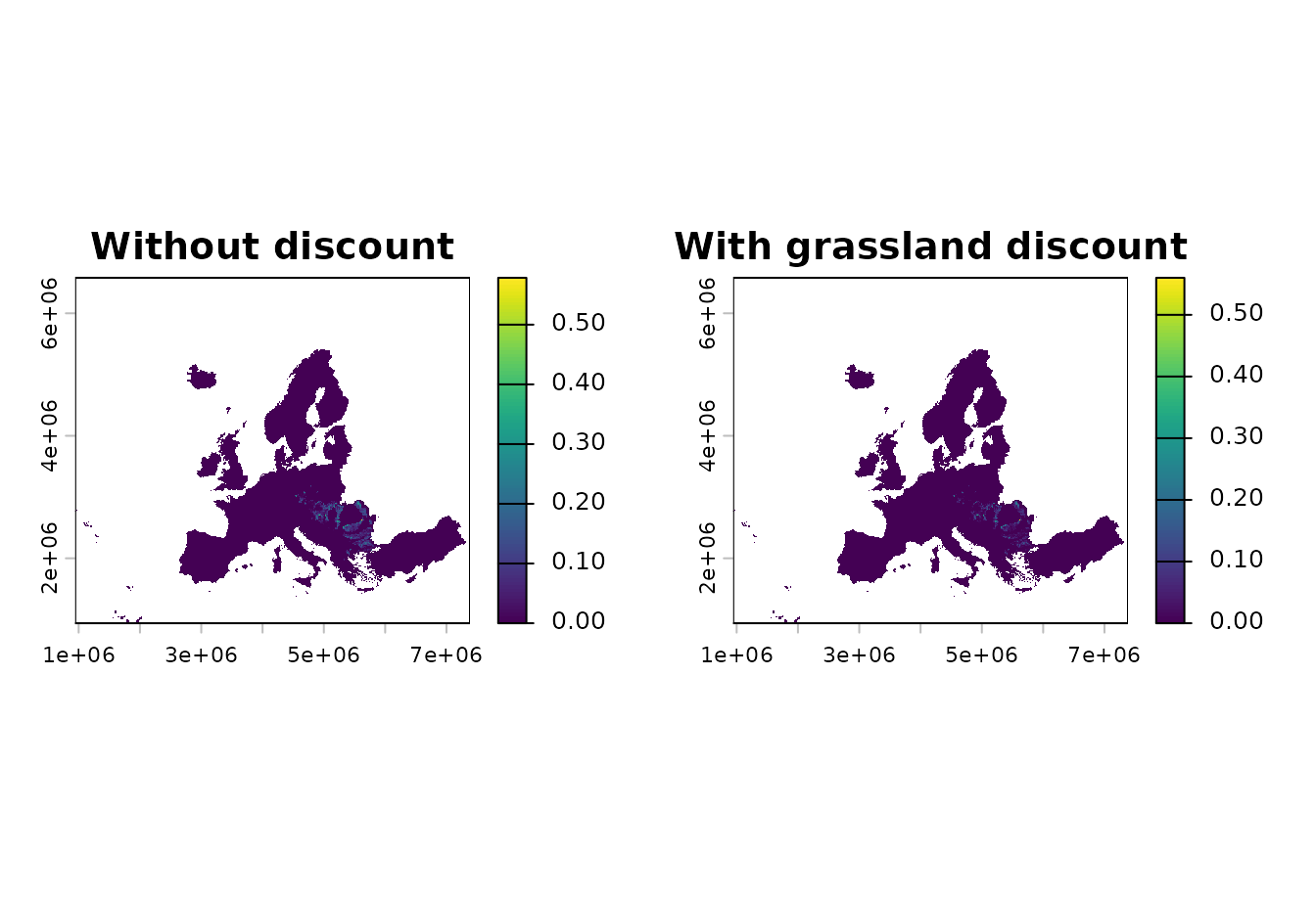

par(op)

insights_summary(aoh_discounted, relative = FALSE)
#>   time suitability unit
#> 1   NA     11646.5  km2

Indicators: `insights_summary()`

With a single-layer raster, insights_summary() reports an absolute total. With multiple layers or time steps, it can also report change relative to the first time step. The standard relative change and symmetric relative change are both returned as fractions; the symmetric relative change is bounded in [-1, 1].

aoh_series <- c(aoh_fraction, aoh_discounted, aoh_discounted * 0.8)
names(aoh_series) <- c("baseline", "maturity_discount", "future_example")
terra::time(aoh_series, tstep = "years") <- c(2020, 2040, 2060)

index_summary <- insights_summary(
  aoh_series,
  relative = TRUE,
  symmetric = TRUE
)
index_summary
#>   time suitability unit relative_change relative_change_sym
#> 1 2020        0.00  km2       0.0000000           0.0000000
#> 2 2040   -11944.22  km2      -0.5063101          -0.3389660
#> 3 2060   -14273.52  km2      -0.6050481          -0.4337412

plot(
  index_summary$time,
  index_summary$relative_change,
  type = "b",
  pch = 19,
  xlab = "Year",
  ylab = "Relative change",
  main = "InSiGHTS index relative to 2020"
)
abline(h = 0, lty = 2, col = "grey50")

Temporal scenario example

The package also ships a small temporal scenario for Bombina bombina. This is a stars object with a time dimension and an ensemble_threshold attribute. It is useful for demonstrating how the insights_*() functions handle temporal range inputs.

bombina_range <- stars::read_mdim(system.file(
  "extdata/Bombina_bombina__ssp126.nc",
  package = "ibis.insights",
  mustWork = TRUE
))
bombina_range <- split(bombina_range)
bombina_range <- bombina_range["ensemble_threshold"]

invisible(utils::capture.output({
  bombina_aoh <- suppressMessages(insights_fraction(
    range = bombina_range,
    lu = lu_fraction,
    clamp = TRUE
  ))
}))

bombina_summary <- insights_summary(
  bombina_aoh,
  relative = TRUE,
  symmetric = TRUE
)
bombina_summary
#>         time       band suitability unit relative_change relative_change_sym
#> 1 2015-01-01 2015-01-01       0.000  km2      0.00000000          0.00000000
#> 2 2025-01-01 2025-01-01   -1760.229  km2     -0.02073683         -0.01047704
#> 3 2035-01-01 2035-01-01   -9637.467  km2     -0.11353665         -0.06018492
#> 4 2045-01-01 2045-01-01   -7887.350  km2     -0.09291895         -0.04872312
#> 5 2055-01-01 2055-01-01   -9587.168  km2     -0.11294409         -0.05985201
#> 6 2065-01-01 2065-01-01  -13247.307  km2     -0.15606329         -0.08463593
#> 7 2075-01-01 2075-01-01  -12746.687  km2     -0.15016560         -0.08117786
#> 8 2085-01-01 2085-01-01  -15312.780  km2     -0.18039612         -0.09914033
#> 9 2095-01-01 2095-01-01  -16806.513  km2     -0.19799342         -0.10987386

bombina_aoh_raster <- terra::rast(bombina_aoh)
terra::time(bombina_aoh_raster) <- stars::st_get_dimension_values(
  bombina_aoh,
  "time"
)

op <- par(mfrow = c(1, 3), mar = c(2, 2, 3, 4))
plot(bombina_aoh_raster[[1]], main = "2015")
plot(bombina_aoh_raster[[5]], main = "2055")
plot(bombina_aoh_raster[[9]], main = "2095")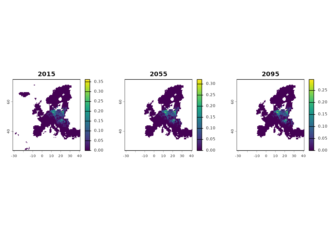

par(op)

plot(
  as.Date(bombina_summary$time),
  bombina_summary$relative_change,
  type = "b",
  pch = 19,
  xlab = "Year",
  ylab = "Relative change",
  main = "Temporal InSiGHTS index"
)
abline(h = 0, lty = 2, col = "grey50")

Example inputs

Fractional land-use: insights_fraction()

Areal land-use: insights_area()

Maturity weighting: insights_discount()

Indicators: insights_summary()

Temporal scenario example

Fractional land-use: `insights_fraction()`

Areal land-use: `insights_area()`

Maturity weighting: `insights_discount()`

Indicators: `insights_summary()`