2) ibis.iSDM integration • ibis.insights

This article shows the direct ibis.iSDM integration points in ibis.insights. Direct ibis object support is intentionally limited to insights_fraction() and insights_area(), where the thresholded distribution or projection layer is used. Other preparation steps, such as maturity discounting or using a continuous suitability projection, should operate on SpatRaster or stars objects before combining them with ibis outputs.

The examples fit a small ibis.iSDM model with the example data distributed by ibis.iSDM, threshold it, project it to a future predictor cube, and then apply the InSiGHTS methods directly to the resulting ibis objects.

library(ibis.insights)
library(ibis.iSDM)
library(terra)
library(stars)
library(sf)

Example Data

The current model is trained from the ibis.iSDM Europe grid, virtual occurrence points, and the first time step of the present-future predictor stack. Land-use inputs for InSiGHTS are built from the crops and secdf predictor layers.

background <- terra::rast(system.file(
  "extdata/europegrid_50km.tif",
  package = "ibis.iSDM",
  mustWork = TRUE
))

sea <- terra::deepcopy(background) != 1
sea[is.na(sea)] <- 1
sea <- terra::as.int(sea)

virtual_range <- sf::st_read(
  system.file("extdata/input_data.gpkg", package = "ibis.iSDM", mustWork = TRUE),
  "range",
  quiet = TRUE
)
virtual_points <- sf::st_read(
  system.file("extdata/input_data.gpkg", package = "ibis.iSDM", mustWork = TRUE),
  "points",
  quiet = TRUE
)

predictor_files <- list.files(
  system.file("extdata/predictors_presfuture/", package = "ibis.iSDM",
              mustWork = TRUE),
  full.names = TRUE
)

suppressWarnings(
  pred_future <- stars::read_stars(predictor_files) |>
    stars:::slice.stars("Time", seq(1, 86, by = 10))
)
sf::st_crs(pred_future) <- sf::st_crs(4326)

pred_current <- ibis.iSDM:::stars_to_raster(pred_future, 1)[[1]]
names(pred_current) <- names(pred_future)

land_use_current <- pred_current[[c("crops", "secdf")]]
land_use_current <- ibis.iSDM::predictor_transform(
  land_use_current,
  option = "norm"
) |>
  round(2)
names(land_use_current) <- c("crops", "secondary_forest")

op <- par(mfrow = c(1, 3), mar = c(2, 2, 3, 4))
plot(background, main = "Model background")
plot(land_use_current[["crops"]], main = "Crops fraction")
plot(land_use_current[["secondary_forest"]], main = "Secondary forest")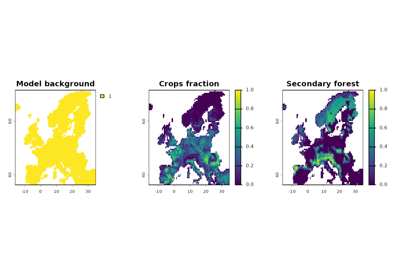

par(op)

Fit And Threshold A Distribution

The fitted object is a real ibis.iSDM DistributionModel. After thresholding, it can be passed directly to insights_fraction() and insights_area().

poa <- virtual_points |>
  add_pseudoabsence(field_occurrence = "Observed", template = background)

distribution_model <- distribution(background) |>
  add_biodiversity_poipa(
    poa,
    field_occurrence = "Observed",
    name = "Virtual points"
  ) |>
  add_predictors(
    pred_current,
    transform = "none",
    derivates = "none"
  ) |>
  engine_glm()

modf <- train(
  distribution_model,
  runname = "Null",
  only_linear = FALSE,
  filter_predictors = "none",
  inference_only = FALSE,
  verbose = FALSE
)
modf <- threshold(modf, method = "perc", value = 0.3)

modf$show_rasters()
#> [1] "prediction"           "threshold_percentile"

modf$plot_threshold()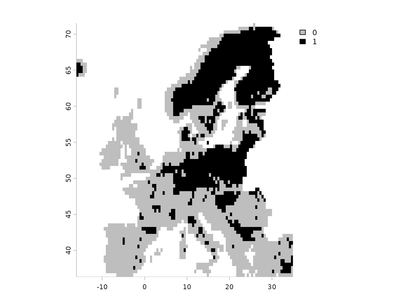

Direct Distribution Methods

Direct DistributionModel calls use the thresholded raster in the ibis object. The land-use layers are summed and applied as fractional habitat layers.

threshold_aoh <- insights_fraction(
  range = modf,
  lu = land_use_current,
  clamp = TRUE
)

insights_summary(threshold_aoh, relative = FALSE)
#>   time suitability unit
#> 1   NA    842020.7  km2

threshold_layer <- modf$get_data("threshold_percentile")
if (terra::nlyr(threshold_layer) > 1) {
  threshold_layer <- threshold_layer[[grep("mean", names(threshold_layer))[1]]]
}
summed_land_use <- terra::app(land_use_current, "sum", na.rm = TRUE)
summed_land_use <- st_clamp(summed_land_use, lb = 0, ub = 1)

op <- par(mfrow = c(1, 3), mar = c(2, 2, 3, 4))
plot(threshold_layer, main = "ibis threshold")
plot(summed_land_use, main = "Suitable land use")
plot(threshold_aoh, main = "Thresholded InSiGHTS")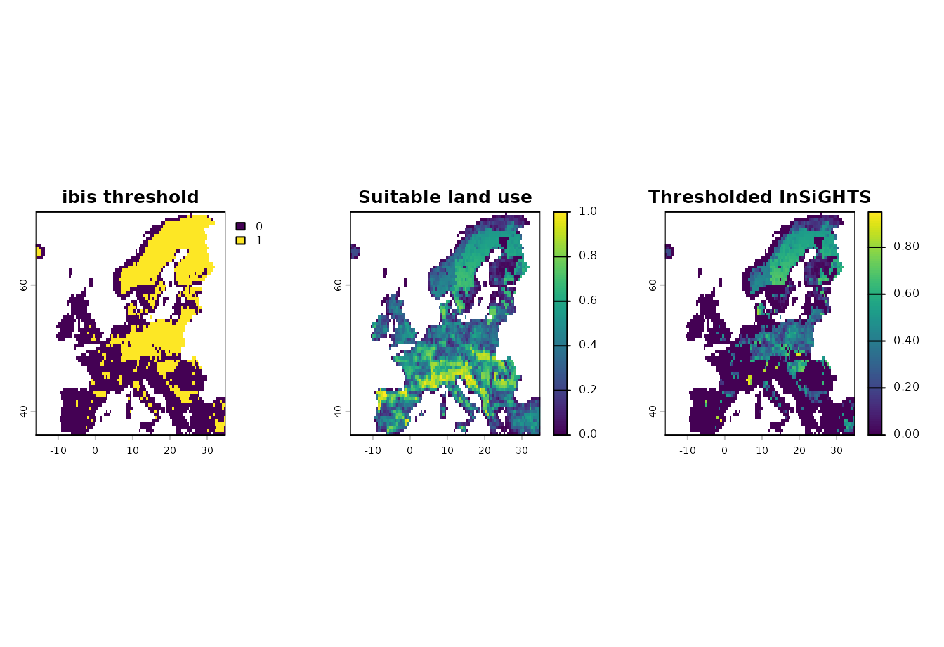

par(op)

Area-valued land-use layers work the same way with insights_area().

land_use_area <- land_use_current * terra::cellSize(
  land_use_current[[1]],
  unit = "km"
)

threshold_area <- insights_area(
  range = modf,
  lu = land_use_area
)

insights_summary(threshold_area, toArea = FALSE, relative = FALSE)
#>   time suitability  unit
#> 1   NA    842020.7 input

Prepared Inputs First

Maturity discounting is a raster operation. Apply it to the land-use layer first, then combine the prepared layer with the ibis object.

forest_age <- land_use_current[["secondary_forest"]] * 40
names(forest_age) <- "secondary_forest_age_years"

invisible(utils::capture.output({
  discounted_forest <- insights_discount(
    lu = land_use_current[["secondary_forest"]],
    age = forest_age,
    target_age = 20,
    target = 0.95
  )
}))
names(discounted_forest) <- "discounted_secondary_forest"

discounted_land_use <- c(land_use_current[["crops"]], discounted_forest)
names(discounted_land_use) <- c("crops", "discounted_secondary_forest")

discounted_aoh <- insights_fraction(
  range = modf,
  lu = discounted_land_use,
  clamp = TRUE
)

rbind(
  no_discount = insights_summary(threshold_aoh, relative = FALSE),
  discounted = insights_summary(discounted_aoh, relative = FALSE)
)
#>             time suitability unit
#> no_discount   NA    842020.7  km2
#> discounted    NA    811157.7  km2

op <- par(mfrow = c(1, 3), mar = c(2, 2, 3, 4))
plot(land_use_current[["secondary_forest"]], main = "Secondary forest")
plot(forest_age, main = "Age proxy")
plot(discounted_forest, main = "Discounted forest")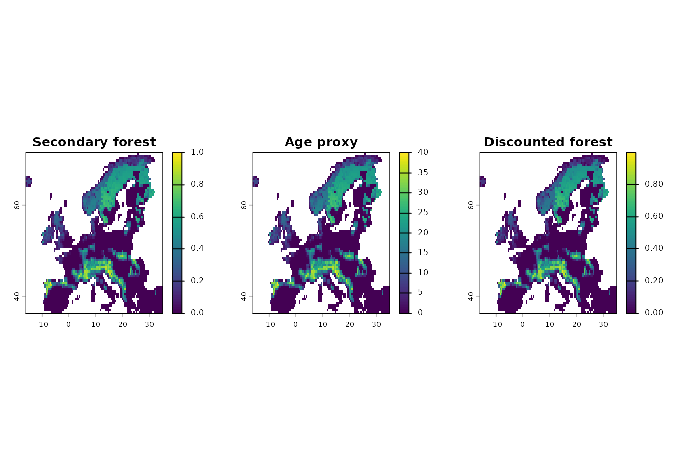

par(op)

Project A Scenario

The scenario projection is a real ibis.iSDM BiodiversityScenario. It is thresholded before projection so the direct InSiGHTS methods can use the projected threshold layer.

mod <- scenario(modf, reuse_limits = FALSE, copy_model = TRUE) |>
  add_predictors(
    env = pred_future,
    transform = "none",
    derivates = "none"
  ) |>
  threshold() |>
  project()

names(mod$get_data())
#> [1] "suitability" "threshold"

For scenario objects, temporal land-use or condition layers with different time steps are aligned to the scenario with align_temporal(). Here the land-use input keeps only the first and final time steps, while the scenario projection contains all projected time steps.

land_use_future <- pred_future |>
  stars:::select.stars(crops, secdf) |>
  stars:::slice.stars("Time", c(1, 9))
land_use_future <- ibis.iSDM::predictor_transform(
  land_use_future,
  option = "norm"
) |>
  round(2)
#> [Setup] 2026-06-14 15:07:39.302828 | When transforming future variables, ensure that unit ranges are comparable (parameter state)!
names(land_use_future) <- c("crops", "secondary_forest")

stars::st_get_dimension_values(land_use_future, "Time")
#> NULL

scenario_aoh <- insights_fraction(
  range = mod,
  lu = land_use_future,
  clamp = TRUE
)

scenario_summary <- insights_summary(
  scenario_aoh,
  relative = TRUE,
  symmetric = TRUE
)
scenario_summary
#>         time       band suitability unit relative_change relative_change_sym
#> 1 2015-01-01 2015-01-01        0.00  km2      0.00000000          0.00000000
#> 2 2025-01-01 2025-01-01   -53922.03  km2     -0.06403884         -0.03307858
#> 3 2035-01-01 2035-01-01  -125891.75  km2     -0.14951146         -0.08079567
#> 4 2045-01-01 2045-01-01  -185600.37  km2     -0.22042256         -0.12386230
#> 5 2055-01-01 2055-01-01  -258136.68  km2     -0.30656808         -0.18103360
#> 6 2065-01-01 2065-01-01  -351191.69  km2     -0.41708199         -0.26348932
#> 7 2075-01-01 2075-01-01  -455024.35  km2     -0.54039566         -0.37023435
#> 8 2085-01-01 2085-01-01  -534150.31  km2     -0.63436717         -0.46452250
#> 9 2095-01-01 2095-01-01  -615340.75  km2     -0.73079050         -0.57578398

scenario_aoh_raster <- terra::rast(scenario_aoh)
scenario_times <- stars::st_get_dimension_values(scenario_aoh, "time")

op <- par(mfrow = c(1, 3), mar = c(2, 2, 3, 4))
plot(scenario_aoh_raster[[1]], main = format(scenario_times[1], "%Y"))
plot(scenario_aoh_raster[[5]], main = format(scenario_times[5], "%Y"))
plot(scenario_aoh_raster[[9]], main = format(scenario_times[9], "%Y"))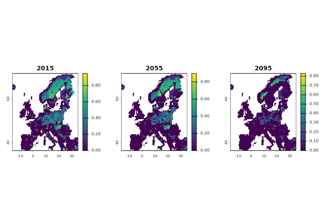

par(op)

plot(
  as.Date(scenario_summary$time),
  scenario_summary$relative_change,
  type = "b",
  pch = 19,
  xlab = "Year",
  ylab = "Relative change",
  main = "Scenario InSiGHTS index"
)
abline(h = 0, lty = 2, col = "grey50")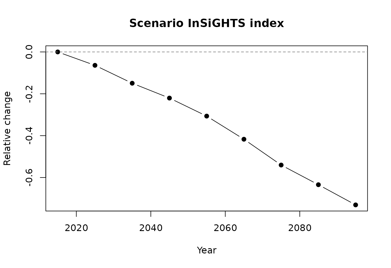

Continuous Suitability

Continuous suitability is not a special ibis dispatch mode in ibis.insights. Extract it from the ibis.iSDM object and pass the resulting SpatRaster or stars object to the normal raster methods.

scenario_layers <- mod$get_data()
suitability_name <- setdiff(names(scenario_layers), "threshold")[1]
suitability_projection <- scenario_layers[suitability_name]
names(suitability_projection) <- "suitability"

suitability_aoh <- insights_fraction(
  range = suitability_projection,
  lu = land_use_future,
  clamp = TRUE
)

insights_summary(suitability_aoh, relative = TRUE)
#>         time       band suitability unit relative_change
#> 1 2015-01-01 2015-01-01        0.00  km2      0.00000000
#> 2 2025-01-01 2025-01-01   -26412.91  km2     -0.02409323
#> 3 2035-01-01 2035-01-01   -59455.48  km2     -0.05423389
#> 4 2045-01-01 2045-01-01   -96997.94  km2     -0.08847923
#> 5 2055-01-01 2055-01-01  -141190.15  km2     -0.12879032
#> 6 2065-01-01 2065-01-01  -187187.09  km2     -0.17074764
#> 7 2075-01-01 2075-01-01  -230156.64  km2     -0.20994346
#> 8 2085-01-01 2085-01-01  -273804.68  km2     -0.24975816
#> 9 2095-01-01 2095-01-01  -311189.54  km2     -0.28385976

Use the thresholded workflow when a binary area of habitat is required, and use an extracted suitability workflow when the climatic suitability value should remain part of the final index.