Niche plot for distribution objects

The suitability of any given area for a biodiversity feature can in many instances be complex and non-linear. Visualizing obtained suitability predictions (e.g. from train()) against underlying predictors might help to explain the underlying gradients of the niche.

Supported Inputs for this function are either single trained ibis.iSDM DistributionModel objects or alternatively a set of three SpatRaster objects. In both cases, users can specify "xvar" and "yvar" explicitly or leave them empty. In the latter case a principal component analysis (PCA) is conducted on the full environmental stack (loaded from DistributionModel or supplied separately).

Usage

nicheplot(
  mod,
  xvar = NULL,
  yvar = NULL,
  envvars = NULL,
  overlay_data = FALSE,
  plot = TRUE,
  fname = NULL,
  title = NULL,
  pal = NULL,
  ...
)

# S4 method for class 'ANY'
nicheplot(
  mod,
  xvar = NULL,
  yvar = NULL,
  envvars = NULL,
  overlay_data = FALSE,
  plot = TRUE,
  fname = NULL,
  title = NULL,
  pal = NULL,
  ...
)

Arguments

mod

A trained DistributionModel or alternatively a SpatRaster object with prediction model within.

xvar

A character denoting the predictor on the x-axis. Alternatively a SpatRaster object can be provided.

yvar

A character denoting the predictor on the y-axis. Alternatively a SpatRaster object can be provided.

envvars

A SpatRaster object containing all environmental variables. Only used if xvar and yvar is empty (Default: NULL).

overlay_data

A logical on whether training data should be overlaid on the plot. Only used for DistributionModel objects (Default: FALSE).

plot

A logical indication of whether the result is to be plotted (Default: TRUE)?

fname

A character specifying the output file name a created figure should be written to.

title

Allows to respecify the title through a character (Default: NULL).

pal

An optional vector with continuous custom colours (Default: NULL).

...

Other engine specific parameters.

Value

Saved niche plot in 'fname' if specified, otherwise plot.

See also

partial, plot.DistributionModel

Examples

# Make quick prediction
background <- terra::rast(system.file('extdata/europegrid_50km.tif',
package='ibis.iSDM',mustWork = TRUE))
virtual_points <- sf::st_read(system.file('extdata/input_data.gpkg', package='ibis.iSDM'), 'points',quiet = TRUE)
ll <- list.files(system.file('extdata/predictors/',package = 'ibis.iSDM',mustWork = TRUE),full.names = TRUE)

# Load them as rasters
predictors <- terra::rast(ll);names(predictors) <- tools::file_path_sans_ext(basename(ll))

# Add GLM as an engine and predict
fit <- distribution(background) |>
add_biodiversity_poipo(virtual_points, field_occurrence = 'Observed',
name = 'Virtual points',docheck = FALSE) |>
add_predictors(predictors, transform = 'none',derivates = 'none') |>
engine_glm() |>
train()
#> [Setup] 2025-06-19 20:45:10.216871 | Creating distribution object...
#> [Setup] 2025-06-19 20:45:10.217789 | Adding poipo dataset...
#> [Setup] 2025-06-19 20:45:10.223161 | Adding predictors...
#> [Estimation] 2025-06-19 20:45:10.408863 | Collecting input parameters.
#> [Estimation] 2025-06-19 20:45:10.56832 | Adding engine-specific parameters.
#> [Estimation] 2025-06-19 20:45:10.572564 | Engine setup.
#> [Estimation] 2025-06-19 20:45:10.789128 | Starting fitting: Virtual points
#> [Estimation] 2025-06-19 20:45:10.852419 | Starting prediction...
#> [Done] 2025-06-19 20:45:10.983861 | Completed after 0.57 secs

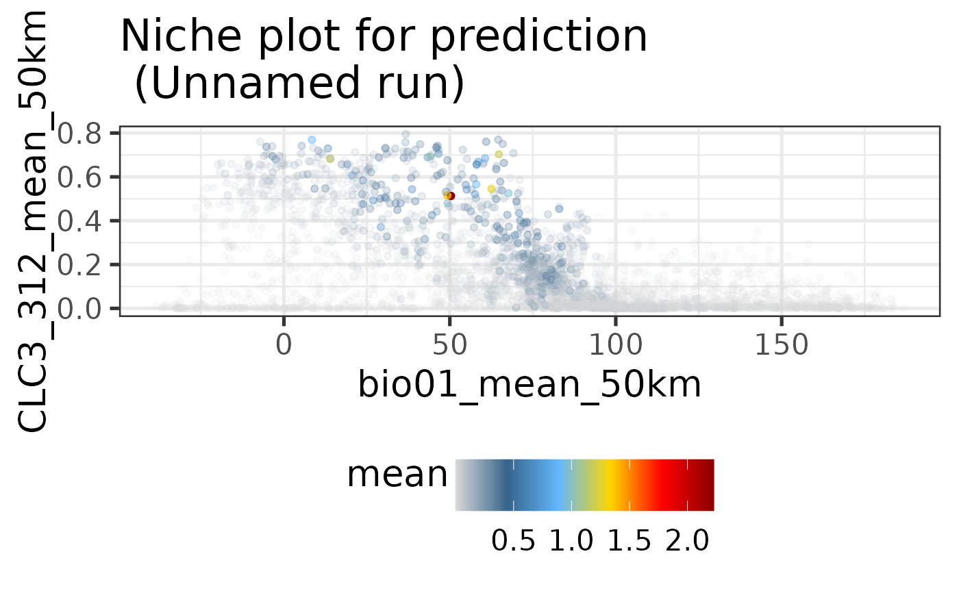
# Plot niche for prediction for temperature and forest cover
nicheplot(fit, xvar = "bio01_mean_50km", yvar = "CLC3_312_mean_50km" )