Data integration
Martin Jung
2026-06-15
Source:vignettes/articles/03_integrate_data.Rmd
03_integrate_data.RmdOne of the key ambitions of the ibis.iSDM R-package is
to provide a comprehensive framework for model-based integration of
different biodiversity datasets and parameters. As ‘integration’ in the
context of SDMs we generally refer to as any approach where additional
observational data or parameters find their way into model estimation.
The purpose behind the integration can be:
- to correct for certain biases (spatial, environmental) in the primary dataset, taking advantage of different types of biodiversity sampling schemes.
- nudge data-driven algorithms towards estimates that are informed by domain knowledge (through offsets or priors) rather than letting the algorithm making naive uniformly distributed guesses.
- to provide a more comprehensive estimate of the distribution of a species distribution by relying on multiple sources of evidence. Particular when there are multiple surveys that complement each other.
There are thus multiple types of integration and we recommend to have a look at Fletcher et al. (2019) and Isaac et al. (2020) for an overview.
The Package comparison page and the examples below provide some insight into what is currently possible with regards to data integration in the ibis.iSDM R-package. Additional methods, priors and engines are planned. Of course it is equally possible to ‘integrate’ not only observational data and parameters, but link entire models with ibis.iSDM outputs. More on this in the scenario help page.
Load relevant packages and testing data
# Load the package
library(ibis.iSDM)
library(inlabru)
library(glmnet)
library(xgboost)
library(terra)
library(igraph)
library(assertthat)

# Don't print out as many messages
options("ibis.setupmessages" = FALSE)
Lets load some of the prepared test data for this exercise. This time we are going to make use of several datasets.
# Background layer
background <- terra::rast(system.file("extdata/europegrid_50km.tif",package = "ibis.iSDM", mustWork = TRUE))
# Load virtual species points
virtual_species <- sf::st_read(system.file("extdata/input_data.gpkg",package = "ibis.iSDM", mustWork = TRUE), "points", quiet = TRUE)
virtual_range <- sf::st_read(system.file('extdata/input_data.gpkg', package='ibis.iSDM'), 'range', quiet = TRUE)

# In addition we will use the species data to generate a presence-absence dataset with pseudo-absence points.
# Here we first specify the settings to use:
ass <- pseudoabs_settings(background = background, nrpoints = 200,
                          method =  "random")
virtual_pseudoabs <- add_pseudoabsence(df = virtual_species, field_occurrence = "Observed",
                                       settings = ass)

# Predictors
predictors <- terra::rast(list.files(system.file("extdata/predictors/", package = "ibis.iSDM", mustWork = TRUE), "*.tif",full.names = TRUE))
# Make use only of a few of them
predictors <- subset(predictors, c("bio01_mean_50km","bio03_mean_50km","bio19_mean_50km",
                                            "CLC3_112_mean_50km","CLC3_132_mean_50km",
                                            "CLC3_211_mean_50km","CLC3_312_mean_50km",
                                            "elevation_mean_50km"))
We can define a generic model to use for any of the sections below.
# First define a generic model and engine using the available predictors
basemodel <- distribution(background) |>
      add_predictors(env = predictors, transform = "scale", derivates = "none") |>
      engine_inlabru()
Integration through predictors
The most simple way of integrating prior observations into species
distribution models is to add them as covariate. This is based on the
assumption that for instance an expert-drawn range map can be useful in
predicting where species exist might or might not find suitable habitat
(see for instance Domisch et al. 2016).
A benefit of this approach is that predictors can be easily added to all
kinds of engines in the ibis.iSDM package and also used for
scenarios.
# Here we simply add the range as simple binary predictor
mod1 <- basemodel |>
  add_predictor_range(virtual_range, method = "distance")

# We can see that the range has been added to the predictors object
# 'distance_range'
mod1$get_predictor_names()
#> [1] "bio01_mean_50km"     "bio03_mean_50km"     "bio19_mean_50km"
#> [4] "CLC3_112_mean_50km"  "CLC3_132_mean_50km"  "CLC3_211_mean_50km"
#> [7] "CLC3_312_mean_50km"  "elevation_mean_50km" "range_distance"
Expert-ranges can currently be added as simple binary or
distance transform. For the latter more options are
available in the bossMaps R-package as described in Merow et al. 2017.
Another option that has been added is the possibility to add thresholded masks based on some elevational (or other) limits. The idea here is to generate two layers, one with areas between a lower and an upper range and one above the upper range. Regression against such thresholded layers can thus approximate the lower and upper bounds. For instance suppose a species is known to occur between 300 and 800m above sea level, this can be added as follows:
# Specification
basemodel <- distribution(background) |>
      add_predictors(env = predictors, transform = "scale", derivates = "none")  |>
      engine_inlabru()

mod1 <- basemodel |>
  add_predictor_elevationpref(layer = predictors$elevation_mean_50km,
                              lower = 300, upper = 800)

# Plot the threshold for an upper
plot( mod1$predictors$get_data()[[c("elev_low", "elev_high")]] )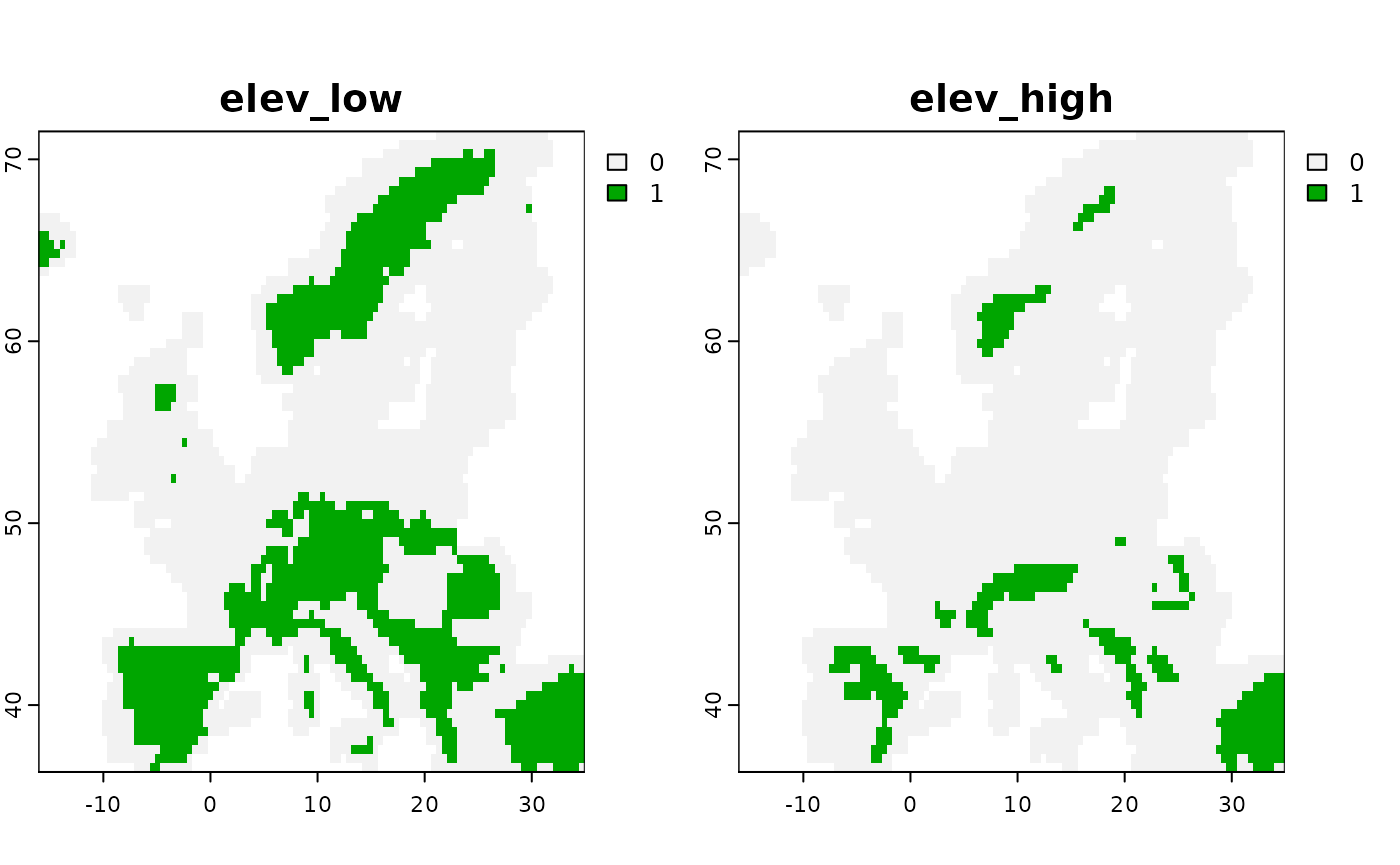
Integration through offsets
Apart from including spatial-explicit prior biodiversity knowledge as predictors in a SDM model, there is - particular for Poisson Process Models (PPM) - also a different approach, that is to include the variable as offset in the prediction. Doing so effectively tells the respective engine to change intercepts and coefficients based on existing knowledge, which can for instance be an existing coefficient. Offsets can be specified as addition or as nuisance for a model, for instance either by adding an expert-delineated range as offset or by factoring out the spatial bias of areas with high sampling density or accessibility. Multiple offsets can be specified for any given PPM by simply multiplying them, since . A comprehensive overview of including offsets in SDMs can be found in Merow et al. (2016).
# Specification
mod1 <- distribution(background)  |>
      add_predictors(env = predictors, transform = "scale", derivates = "none")  |>
      add_biodiversity_poipo(virtual_species,field_occurrence = "Observed") |>
      add_offset_range(virtual_range, distance_max = 5e5) |>
      engine_glmnet() |>
  # Train
  train(runname = "Prediction with range offset",only_linear = TRUE)

plot(mod1)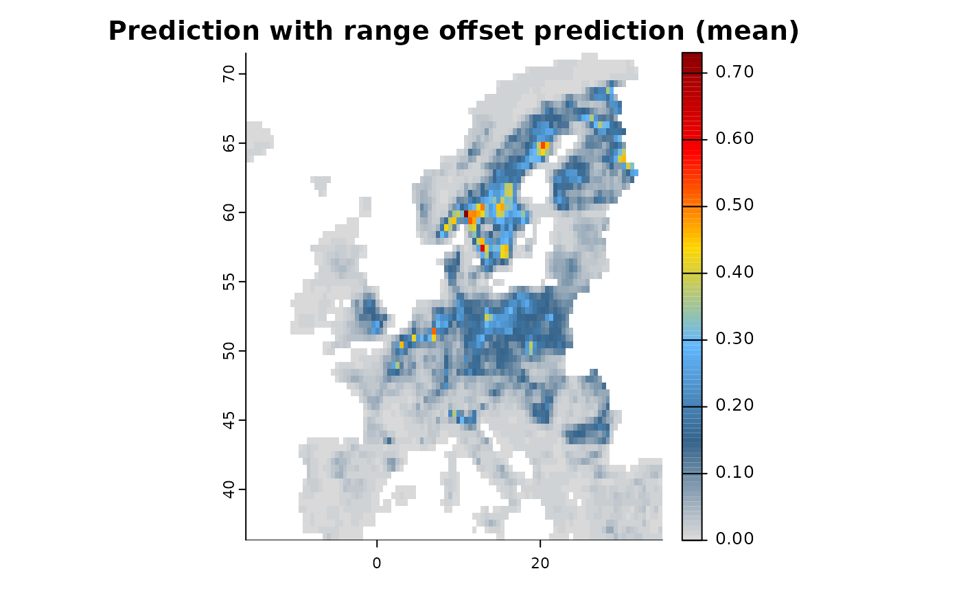
There are other ways to add offsets to the model object, either
directly (add_offset()) as an externally calculated
RasterLayer for instance with the “BossMaps” R-package, to calculate as
range (add_offset_range()) or elevation
(add_offset_elevation()) offset, or also as biased offset
(add_offset_bias()) in which case the offset is removed
from the prediction.
Integration through bias control
Sampling bias is a ubiquitous problem in presence-only biodiversity
data, where observations are often clustered near roads, cities, or
popular natural sites. The add_control_bias() function
allows you to specify a covariate that accounts for this spatial bias
and partial it out of the prediction. The bias_value
parameter sets the value at which the bias covariate is held constant
during prediction (e.g., 0 to represent minimal bias).
# Load a human modification index layer as proxy for sampling bias
bias_layer <- terra::rast(system.file("extdata/predictors/hmi_mean_50km.tif",
                                       package = "ibis.iSDM", mustWork = TRUE))

# Train a model with bias control
mod_bias <- distribution(background) |>
      add_predictors(env = predictors, transform = "scale", derivates = "none") |>
      add_biodiversity_poipo(virtual_species, field_occurrence = "Observed") |>
      # Add bias control: partial out the human modification index during prediction
      add_control_bias(layer = bias_layer, bias_value = 0) |>
      engine_glmnet() |>
      train(runname = "Prediction with bias control", only_linear = TRUE)

plot(mod_bias)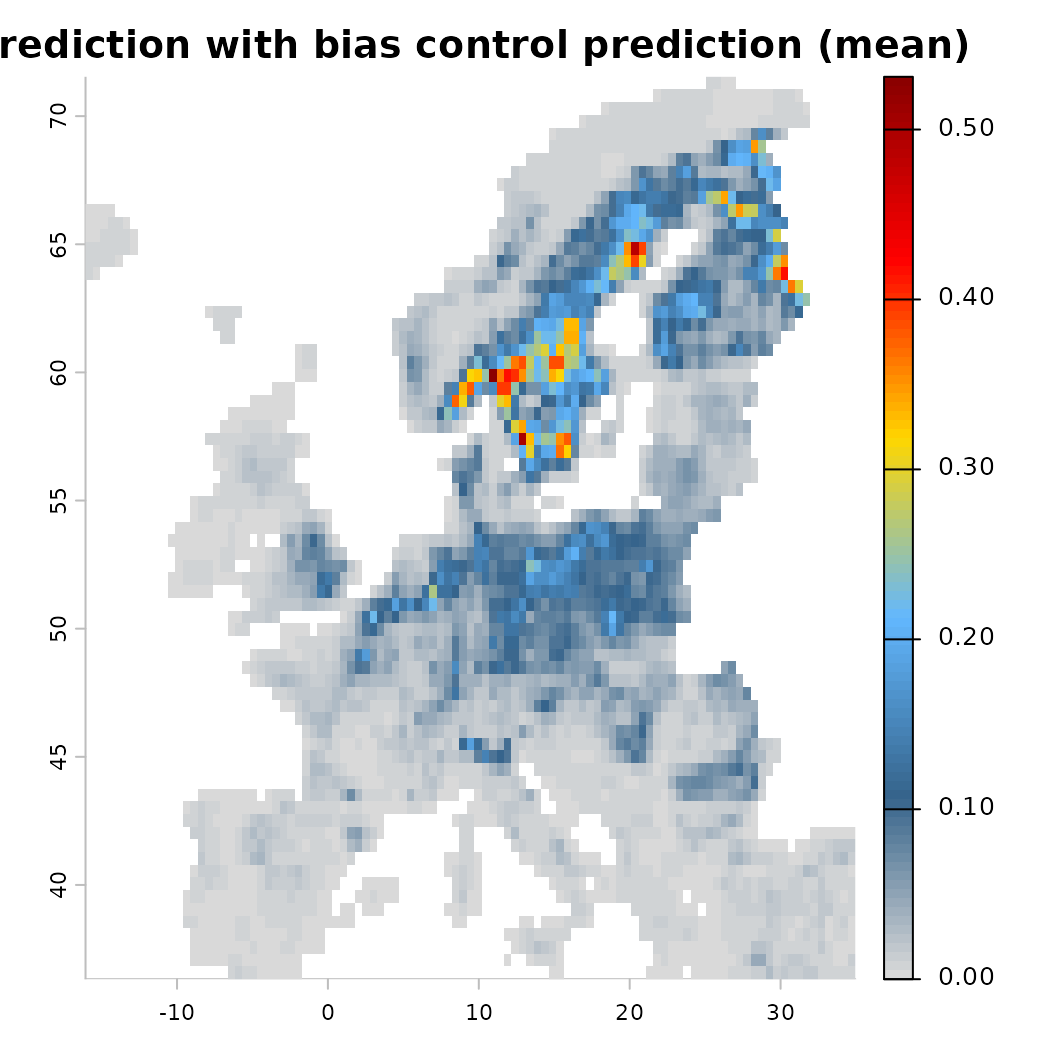
Integration through Ensemble of Small Models (ESM)
When there are very few observations relative to the number of
predictors, fitting a full model can lead to overfitting. The Ensemble
of Small Models (ESM) approach (Breiner et al. 2015)
addresses this by fitting many bivariate models (one per pair of
predictors) and then combining them into an ensemble. This can be
enabled via add_control_esm().
# Train a model using the ESM approach
mod_esm <- distribution(background) |>
      add_predictors(env = predictors, transform = "scale", derivates = "none") |>
      add_biodiversity_poipo(virtual_species, field_occurrence = "Observed") |>
      # Enable ESM: each bivariate model is trained separately and ensembled
      add_control_esm() |>
      engine_glmnet() |>
      train(runname = "ESM prediction", only_linear = TRUE)
#> Training 28 ESM GLMNET-Engine models with 2 predictors each.
#> [Setup] 2026-06-15 20:12:19.511578 | Replacing currently selected engine.
#>
#> ! Overwriting previously defined engine.

plot(mod_esm)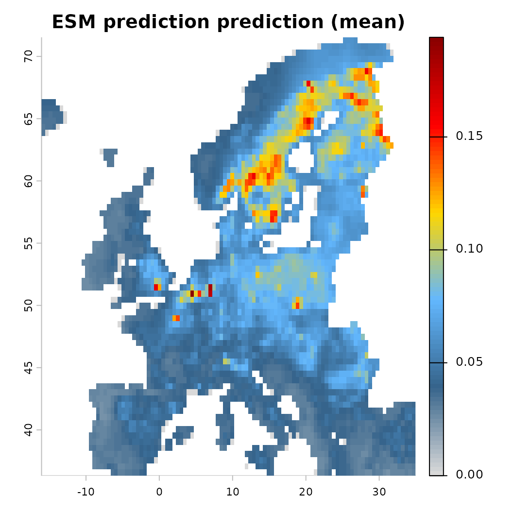
Integration with priors
A different type of integration is also possible through the use of
informed priors, which can be set on fixed or random effects in the
model. In a Bayesian context a prior is generally understood as some
form of uncertain quantity that is meant to reflect the direction and/or
magnitude of model parameters and is usually known a-priori to any
inference or prediction. Offsets can also be understood as “priors”,
however in the context of SDMs, they are usually included as
spatial-explicit data, opposed to priors that are only available in
tabular form (such as known habitat affiliations). Since the ibis.iSDM
package supports a variety of engines and not all of them are Bayesian
in a strict sense (such as engine_gdb or
engine_xgboost), the specification of priors differs
depending on the engine in question.
Generally [Prior-class] objects can be grouped into:
Probabilistic priors with estimates placed on for example the mean () and standard deviation () or precision in the case of [
engine_inla]. Such priors usually allow the greatest amount of flexibility since they are able to incorporate information on both the sign and magnitude of a coefficient.Monotonic constraints on the direction of a coefficient and predictor in the model, such that is or . Useful to incorporate for instance prior ecological knowledge on that a certain response function for example has to be positive.
More complex priors specified on random spatial effects such as penalized complexity priors used for SPDE effects in [
add_latent_spatial()].Probabilistic priors on the inclusion probability of a certain variable such as to what certainty the variable should or should not be included in a regularized outcome. For example used in the case of [
engine_breg] or [engine_glmnet].
Prior specifications are specific to each engine and more information
can be found on the individual help pages of the priors()
function.
# Set a clean base model with biodiversity data
x <- distribution(background) |>
      add_predictors(env = predictors, transform = "scale", derivates = "none") |>
      add_biodiversity_poipo(virtual_species, field_occurrence = "Observed") |>
      engine_inlabru()

# Make a first model
mod1 <- train(x, only_linear = TRUE)
#> Warning: `like()` was deprecated in inlabru 2.12.0.
#> ℹ Please use `bru_obs()` instead.
#> ℹ The deprecated feature was likely used in the ibis.iSDM package.
#>   Please report the issue at <https://github.com/iiasa/ibis.iSDM/issues>.
#> This warning is displayed once per session.
#> Call `lifecycle::last_lifecycle_warnings()` to see where this warning was
#> generated.

# Now assume we now that the species occurs more likely in intensively farmed land.
# We can use this information to construct a prior for the linear coefficient.
p <- INLAPrior(variable = "CLC3_211_mean_50km",
               type = "normal",
               hyper = c(2, 1000) # Precision priors, thus larger sigmas indicate higher precision
               )
# Single/Multiple priors need to be passed to `priors` and then added to the model object.
pp <- priors(p)
# The variables and values in this object can be queried as well
pp$varnames()
#> 7197f0f7-9143-44f0-b30b-796d2e76a53f
#>                 "CLC3_211_mean_50km"

# Priors can then be added via
mod2 <- train(x |> add_priors(pp), only_linear = TRUE)
# Or alternatively directly as parameter via add_predictors,
# e.g. add_predictors(env = predictors, priors = pp)

# Compare the difference in effects
p1 <- partial(mod1, pp$varnames(), plot = TRUE)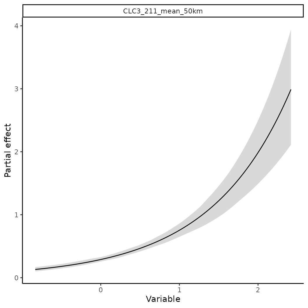
p2 <- partial(mod2, pp$varnames(), plot = TRUE)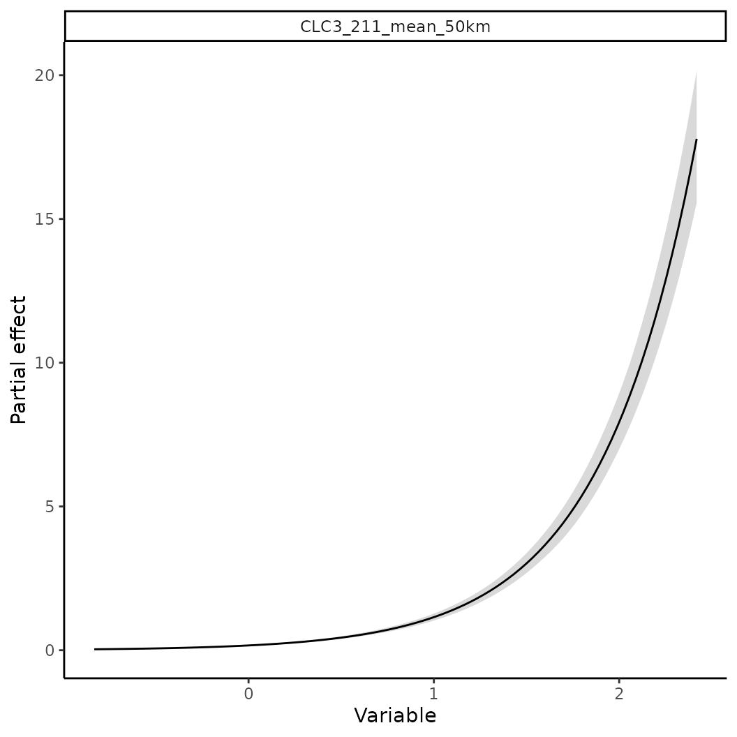
There is also now a convenience function that allows to extract
coefficients or weights from an existing model when can then be passed
to another model or engine (get_priors()). Only requirement
is that a fitted model is provided as well as the target engine for
which coefficients/priors are to be created.
Integration with ensembles
Another very straight forward way for model-based integration is to
simply fit two separate models each with a different biodiversity
dataset and then create an ensemble from them. This approach also works
across different engines and a variety of data types (in some cases
requiring normalization given the difference in units and model
assumptions). (Note that it also possible to create an ensemble of
partial responses via ensemble_partial()).
# Create and fit two models
mod1 <- distribution(background) |>
      add_predictors(env = predictors, transform = "scale", derivates = "none") |>
      engine_glmnet() |>
      # Add dataset 1
      add_biodiversity_poipo(poipo = virtual_species, name = "Dataset1",field_occurrence = "Observed") |>
      train(runname = "Test1", only_linear = TRUE)

mod2 <- distribution(background) |>
      add_predictors(env = predictors, transform = "scale", derivates = "none") |>
      engine_xgboost(iter = 5000) |>
      # Add dataset 2, Here we simple simulate presence-only points from a range
      add_biodiversity_polpo(virtual_range, name = "Dataset2",field_occurrence = "Observed",
                             simulate = TRUE,simulate_points = 300) |>
      train(runname = "Test1", only_linear = FALSE)

# Show outputs of each model individually and combined
plot(mod1)
plot(mod2)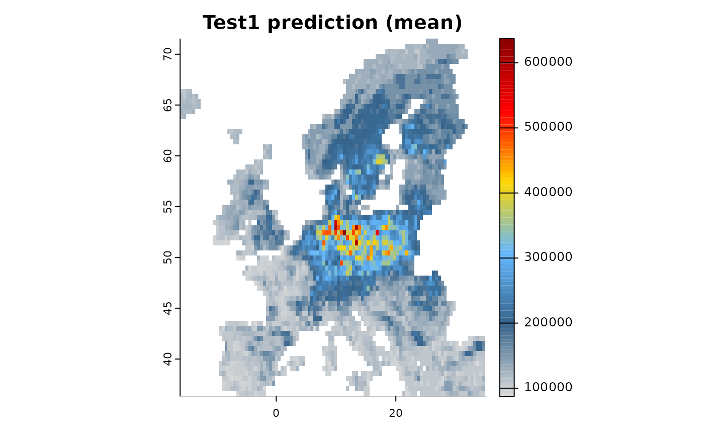
# Now create an ensemble:
# By setting normalize to TRUE we furthermore ensure each prediction
# is on a comparable scale [0-1].
e <- ensemble(mod1, mod2, method = "mean", normalize = TRUE)

# The ensemble contains the mean and the coefficient of variation across all objects
plot(e)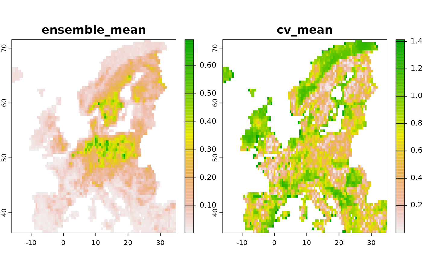
Combined and joint likelihood estimation
In the examples above we always added only a single biodiversity data source to a model to be trained, but what if we add multiple different ones? As outlined by Isaac et al. 2020 joint, model-based integration of different data sources allows to borrow strengths of different types of datasets (quantity, quality) for more accurate parameter estimations as well as the control of biases. Particular for SDMs it also has the benefit of avoiding to make unreasonable assumptions about the absence of a species, as commonly being done through the addition of pseudo-absences (despite being called pseudo, any logistic likelihood function treats them as true absence).
Depending on the engine, the ibis.iSDM package currently supports either combined or joint estimation of several datasets.
Combined integration
By default all engines that do not support any joint estimation (see below) will make use of a combined integration, for which there are currently three different options:
“predictor”: The predicted output of the first (or previously fitted) models are added to the predictor stack and thus are predictors for subsequent models (Default).
“offset”: The predicted output of the first (or previously fitted) models are added as spatial offsets to subsequent models. Offsets are back-transformed depending on the model family. This might not work for all likelihood functions and engines!
“prior”: In this option we only make use of the coefficients from a previous model to define priors to be used in the next model. Note that this option creates priors based on previous fits and can result in unreasonable constrains (particular if coefficients are driven largely by latent variables). Can be used in projections (
scenario()).“interaction”: In the case of two datasets of the same type it also is possible to make use of factor interactions. In this case the prediction is made based on the first reference level (e.g. the first added dataset) with the others being “partialed” out during prediction. This method only works if one fits a model with multiple datasets on the same response (e.g. Bernoulli distributed). Can be used in projections (
scenario()).“weights”: This type of integration works only for two biodiversity datasets of the same type. Here the datasets are combined into one, however the observations are weighted through a
weightsparameter in each add_biodiversity call. This can be for example used to give one dataset an arbitrary (or expert-defined) higher value compared to another.
All of these can be specified as parameter in
train().
Note that for any of these methods (like “predictor” & “offset”), models are trained in the sequence at which datasets are added!
# Specification
mod1 <- distribution(background) |>
      add_predictors(env = predictors, transform = "scale", derivates = "none") |>
    # A presence only dataset
      add_biodiversity_poipo(virtual_species,field_occurrence = "Observed") |>
    # A Presence absence dataset
      add_biodiversity_poipa(virtual_pseudoabs,field_occurrence = "Observed") |>
      engine_xgboost() |>
  # Train
  train(runname = "Combined prediction",only_linear = TRUE,
        method_integration = "predictor")

# The resulting object contains only the final prediction, e.g. that of the presence-absence model
plot(mod1)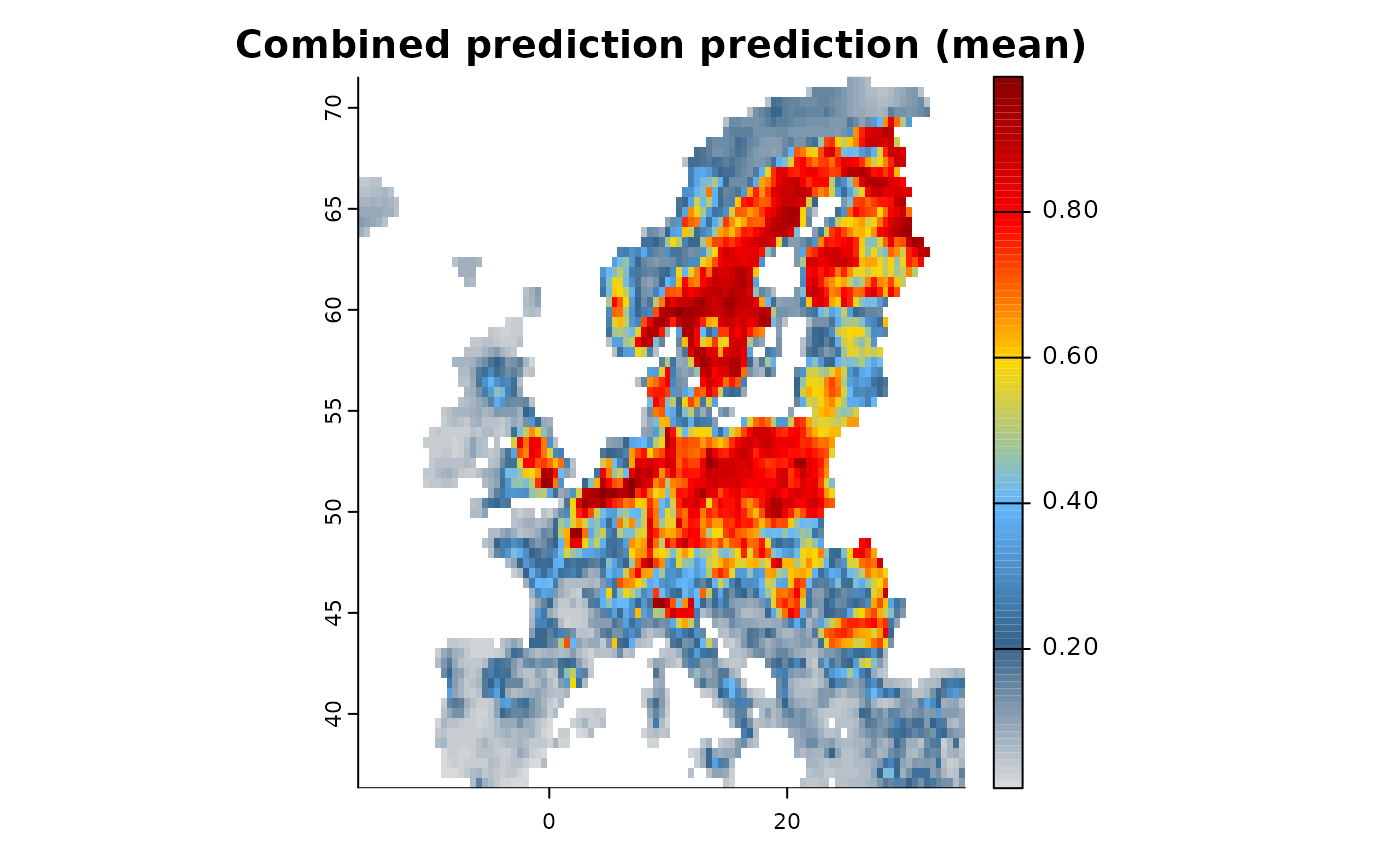
Joint likelihood estimation
Some engines, notably [engine_inla],
[engine_inlabru] and [engine_stan] support the
joint estimation of multiple likelihoods. The algorithmic approach in
this package generally follows an approach outlined where any
presence-only datasets are modelled through a log-Gaussian Cox process
where the expected number of individuals are estimated as a function of
area
following a Poisson distribution:
$$\begin{align*} N(A) &\sim {\sf Poisson}\left(\int_{A} \lambda(i)\right) \\ \end{align*}$$
where is the number of individuals, the Area for a given spatial unit , with being an estimate of the relative rate of occurrence per unit area (or ROR). is an increment for number of predictors. is the intensity function, the intercept and the parameter coefficients for environmental covariates. Note that for interactions
Presence-absence data are estimated as draws from a Bernoulli distribution:
$$\begin{align*} Y_{i} &\sim {\sf Bernoulli(p_{i})}, i = 1, 2, ... \\ \end{align*}$$
where is the presence-absence of an record (usually a standardized survey) as sampled from a Bernoulli distribution in a given spatial unit . being the intercept and the parameter coefficients for environmental covariates. The log-likelihood can be understood as cloglog functon.
The Joint likelihood is then estimated by multiplying the two likelihoods from above , where is an individual likelihood, with being shared parameters between the two likelihoods. This works if we assume that . Equally it is also possible to add shared latent spatial effects such as Gaussian fields (approximated through a stochastic partial differential equation (SPDE)) to the model, assuming that there are shared factors - or biases - affecting all datasets.
See the Engine comparison for an overview on which engines support which level of integration.
# Define a model
mod1 <- distribution(background) |>
      add_predictors(env = predictors, transform = "scale", derivates = "none") |>
    # A presence only dataset
      add_biodiversity_poipo(virtual_species,field_occurrence = "Observed") |>
    # A Presence absence dataset
      add_biodiversity_poipa(virtual_pseudoabs,field_occurrence = "Observed") |>
    # Use inlabru for estimation and default parameters.
    # INLA requires the specification of a mesh which in this example is generated from the data.
      engine_inlabru() |>
  # Train
  train(runname = "Combined prediction", only_linear = TRUE)

# The resulting object contains the combined prediction with shared coefficients among datasets.
plot(mod1)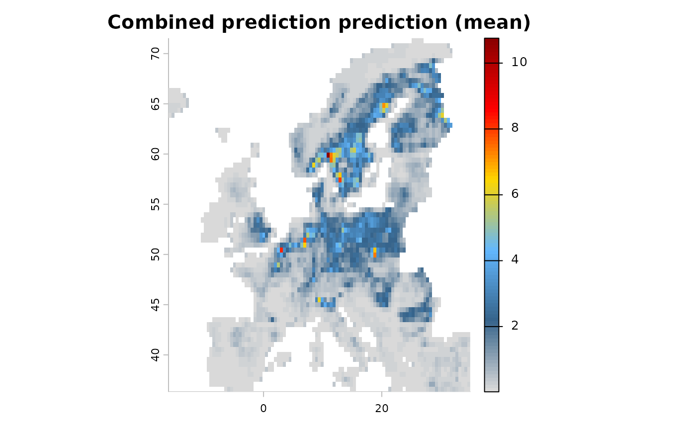
# Note how an overall intercept as well as separate intercepts for each dataset are added.
summary(mod1)
#> # A tibble: 11 × 8
#>    variable                   mean      sd      q05     q50    q95    mode   kld
#>    <chr>                     <dbl>   <dbl>    <dbl>   <dbl>  <dbl>   <dbl> <dbl>
#>  1 Intercept               -0.328  25.8    -42.8    -0.328  42.1   -0.328      0
#>  2 Intercept_X7f79f2ca_po… -0.328  25.8    -42.8    -0.328  42.1   -0.328      0
#>  3 Intercept_X4d95674e_po… -0.328  25.8    -42.8    -0.328  42.1   -0.328      0
#>  4 bio01_mean_50km         -0.109   0.134   -0.330  -0.109   0.112 -0.109      0
#>  5 bio03_mean_50km         -0.482   0.121   -0.681  -0.482  -0.283 -0.482      0
#>  6 bio19_mean_50km          0.472   0.0870   0.329   0.472   0.615  0.472      0
#>  7 CLC3_112_mean_50km       0.407   0.0496   0.325   0.407   0.488  0.407      0
#>  8 CLC3_132_mean_50km       0.0620  0.0496  -0.0197  0.0620  0.144  0.0620     0
#>  9 CLC3_211_mean_50km       0.898   0.0787   0.768   0.898   1.03   0.898      0
#> 10 CLC3_312_mean_50km       0.989   0.0660   0.880   0.989   1.10   0.989      0
#> 11 elevation_mean_50km      0.0251  0.0852  -0.115   0.0251  0.165  0.0251     0