Creating biodiversity projections
Martin Jung
2023-08-25
Source:vignettes/articles/03_biodiversity_projections.Rmd
03_biodiversity_projections.RmdBesides inferring environmental responses and mapping the contemporary distribution of any species (see Train simple Model), species distribution models (SDMs) are commonly used to make predictions on how biodiversity is expected to change under future conditions. Usually this is being done by first training a model on present observations and then projecting the resulting \(\beta\) coefficients to another set of environmental predictors from another time period or spatial region.
The ibis.iSDM R-package provides direct support for
creating such projections. This requires a previously fitted
[DistributionModel] and a new set of covariates which match
in names the covariates on which the fitted model was trained. The key
functions here are scenario() and project()
which are specific to such projections and result in the creation of a
[BiodiversityScenario] object. For other functions the same
syntax as for previously trained models applies, e.g. new predictor can
be added via add_predictors() or thresholds applied via
threshold(). In addition the ibis.iSDM
R-package allows the specification of a number of constrains on the
projections, such as for instance dispersal constrains based on the
expected or simulated chance of individuals dispersing to neighbouring
grid cells. Such constrains can be added via
add_constrain() (and other constrain functionalities in
add_constrain_*()).
Note: Projecting relative suitability estimates into conditions other than the observational records for which the SDM was trained comes with a number of assumptions, most importantly that relationships between occurrences and environmental conditions are in equilibrium and similar biases and conditions apply in the future. See Elith et al. (2010) and discussion in Zurell et al. (2016) for an introduction and comparative overview.
Load relevant packages and testing data
# Load the packages
library(ibis.iSDM)
library(stars)
library(xgboost)
library(terra)
library(igraph)
library(ggplot2)
library(ncdf4)
library(assertthat)

# Don't print out as many messages
options("ibis.setupmessages" = FALSE)
For the purpose of this example we are loading some testing data on species distributions as well as contemporary and future predictors. Note the names of predictors used for building a distribution model have to be consistent with those for creating projections!
# Background and biodiversity data
background <- terra::rast(system.file('extdata/europegrid_50km.tif', package='ibis.iSDM'))
virtual_points <- sf::st_read(system.file('extdata/input_data.gpkg', package='ibis.iSDM'), 'points', quiet = TRUE)
# Note we are loading different predictors than in previous examples
# These are in netcdf4 format, a format specific for storing spatial-temporal data including metadata.
ll <- list.files(system.file("extdata/predictors_presfuture/", package = "ibis.iSDM", mustWork = TRUE), "*.nc",full.names = TRUE)
# From those list of predictors are first loading the current ones as raster data
# We are loading only data from the very first, contemporary time step for model fitting
pred_current <- terra::rast()
for(i in ll) suppressWarnings( pred_current <- c(pred_current, terra::rast(i, lyrs = 1) ) )
names(pred_current) <- tools::file_path_sans_ext( basename(ll) )
# Get future predictors
# These we will load in using the stars package and also ignoring the first time step
pred_future <- stars::read_stars(ll) |> stars:::slice.stars('Time', 2:86)
st_crs(pred_future) <- st_crs(4326) # Set projection
# Rename future predictors to those of current
names(pred_future) <- names(pred_current)
# Plot the test data
plot(pred_current['secdf'],
col = colorRampPalette(c("grey20", "orange", "lightgreen", "green"))(10),
main = "Share of secondary vegetation")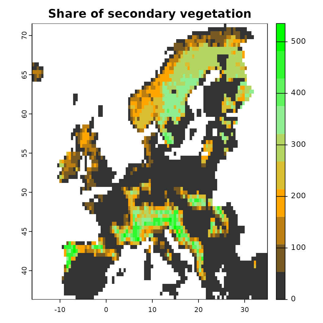 ## Train model and create a future projection
We will make use of the data loaded above to (a) first create a species distribution model for contemporary conditions and (b) project the obtained coefficients into the future using future predictors. For guidance on how distribution models are trained, see other vignettes (1).
# Train model adding the data loaded above
x <- distribution(background) |>
  add_biodiversity_poipo(virtual_points, field_occurrence = 'Observed', name = 'Virtual points') |>
  # Note that we scale the predictors here
  add_predictors(pred_current, transform = 'scale',derivates = 'none') |>
  engine_glmnet(alpha = 0)
#> Loaded glmnet 4.1-8

# Train the model
modf <- train(x, runname = 'Simple PPM', verbose = FALSE)

# Add a threshold to this model by getting 05 percentile of values
modf <- threshold(modf, method = 'percentile', value = 0.05)

# -- #
# Now lets create a scenarios object via scenarios
sc <- scenario(modf) |>
  # Apply the same variable transformations as above.
  add_predictors(pred_future, transform = 'scale') |>
  # Calculate thresholds at each time step. The threshold estimate is taken from the model object.
  threshold()

# This creates a scenario object
sc
#> Spatial-temporal scenario:
#>   Used model: GLMNET-Model
#>  ---------
#>   Predictors:     bio01, bio12, crops, ... (9 predictors)
#>   Time period:    2016-01-01 -- 2100-01-01 (83.9 years)
#>  ---------
#>   Threshold:      0.03 (percentile)
#>  ---------
#>   Scenarios fitted: None
# The object contains its own functions. See the scenarios help file for more information on
# what is possible with them
names(sc)
#>  [1] "constraints"          "get_resolution"       "get_centroid"
#>  [4] "verify"               "get_threshold"        ".super"
#>  [7] "save"                 "modelobject"          "set_constraints"
#> [10] "summary"              "get_timeperiod"       "plot_relative_change"
#> [13] "rm_predictors"        "get_predictors"       "print"
#> [16] "limits"               "apply_threshold"      "predictors"
#> [19] "get_projection"       "get_limits"           "calc_scenarios_slope"
#> [22] "scenarios"            "plot"                 "get_data"
#> [25] "show"                 "modelid"              "summary_beforeafter"
#> [28] "get_predictor_names"  "get_constraints"      "get_model"
#> [31] "set_predictors"       "plot_threshold"       "plot_migclim"
#> [34] ".that"                "plot_animation"       "threshold"
#> [37] "get_thresholdvalue"
The scenario object can finally be trained via
project().
sc.fit1 <- sc |> project()
# Note that an indication of fitted scenarios has been added to the object
sc.fit1
#> Spatial-temporal scenario:
#>   Used model: GLMNET-Model
#>  ---------
#>   Predictors:     bio01, bio12, crops, ... (9 predictors)
#>   Time period:    2016-01-01 -- 2100-01-01 (83.9 years)
#>  ---------
#>   Threshold:      0.03 (percentile)
#>  ---------
#>   Scenarios fitted: Yes
Summarizing and plotting the fitted projections
As with distribution models there are a number of ways how the scenarios can be visualized and interacted with:
-
plot()makes a visualization of the projections over all time steps (!) -
plot_relative_change()calculates the change in suitability area between the first and the last timestep and categorizes the result accordingly. Note that SDMs as such cannot directly infer colonization or extinction, but only gains or losses of suitable habitat! -
calc_scenarios_slope()calculates the slope (rate of change) across timesteps. Useful for summarizing results -
summary()creates a summary output of the contained scenarios. If athreshold()is specified, this function will summarize the amount of area at each timestep. -
get_data()gets the created scenarios astarsobject (plus thresholds if specified).
# Plot all scenarios. With a large number of predictors this figure will be messy...
plot(sc.fit1) # or sc.fit1$plot()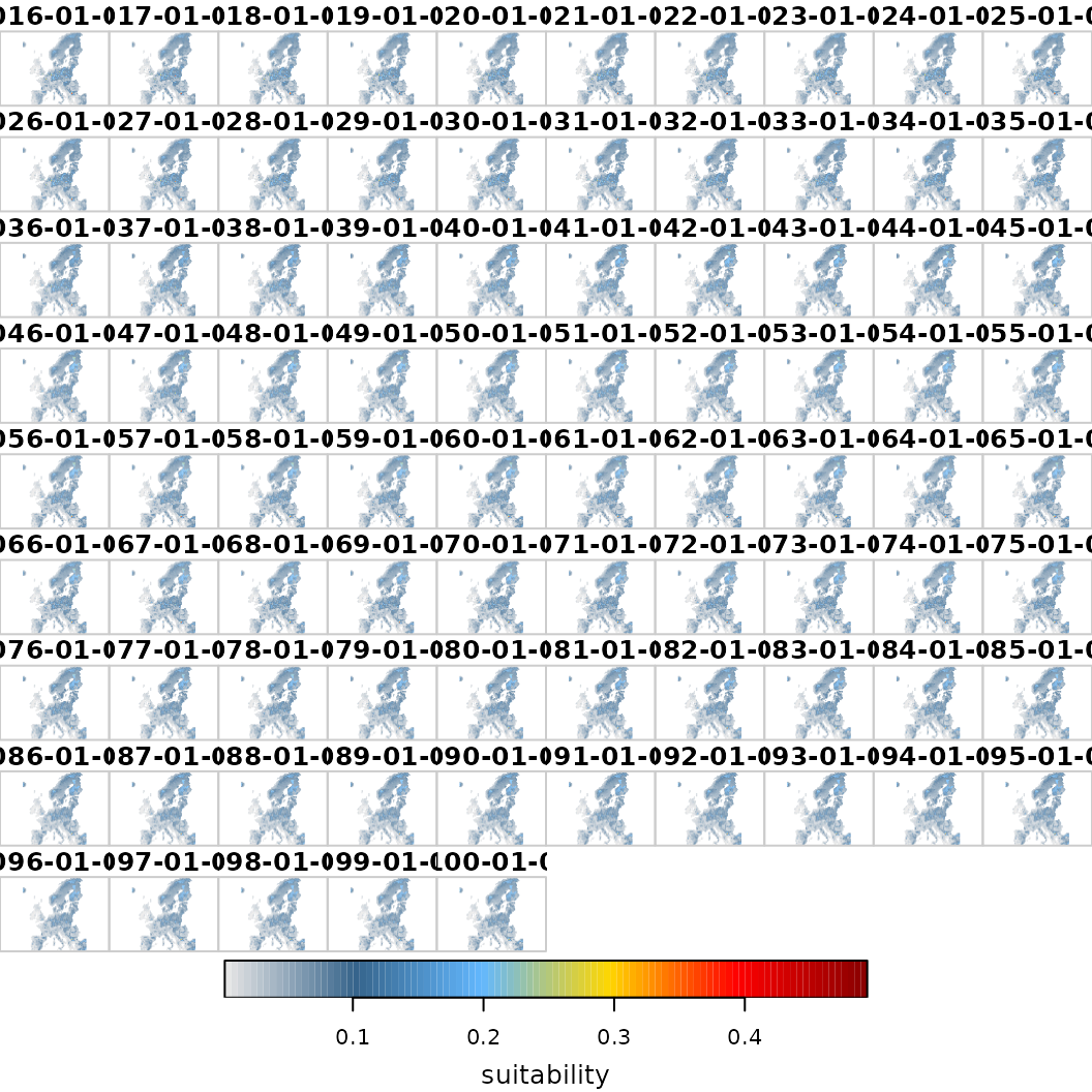
# As an alternative, visualize the linear slope per grid cell and across all time steps
o <- sc.fit1$calc_scenarios_slope(plot = TRUE)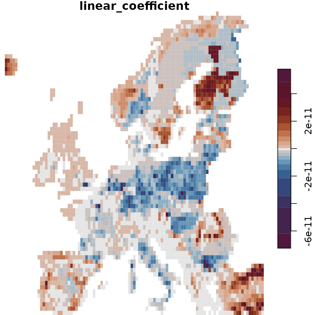
# Another option is to calculate the relative change between start and finish
o <- sc.fit1$plot_relative_change(plot = TRUE)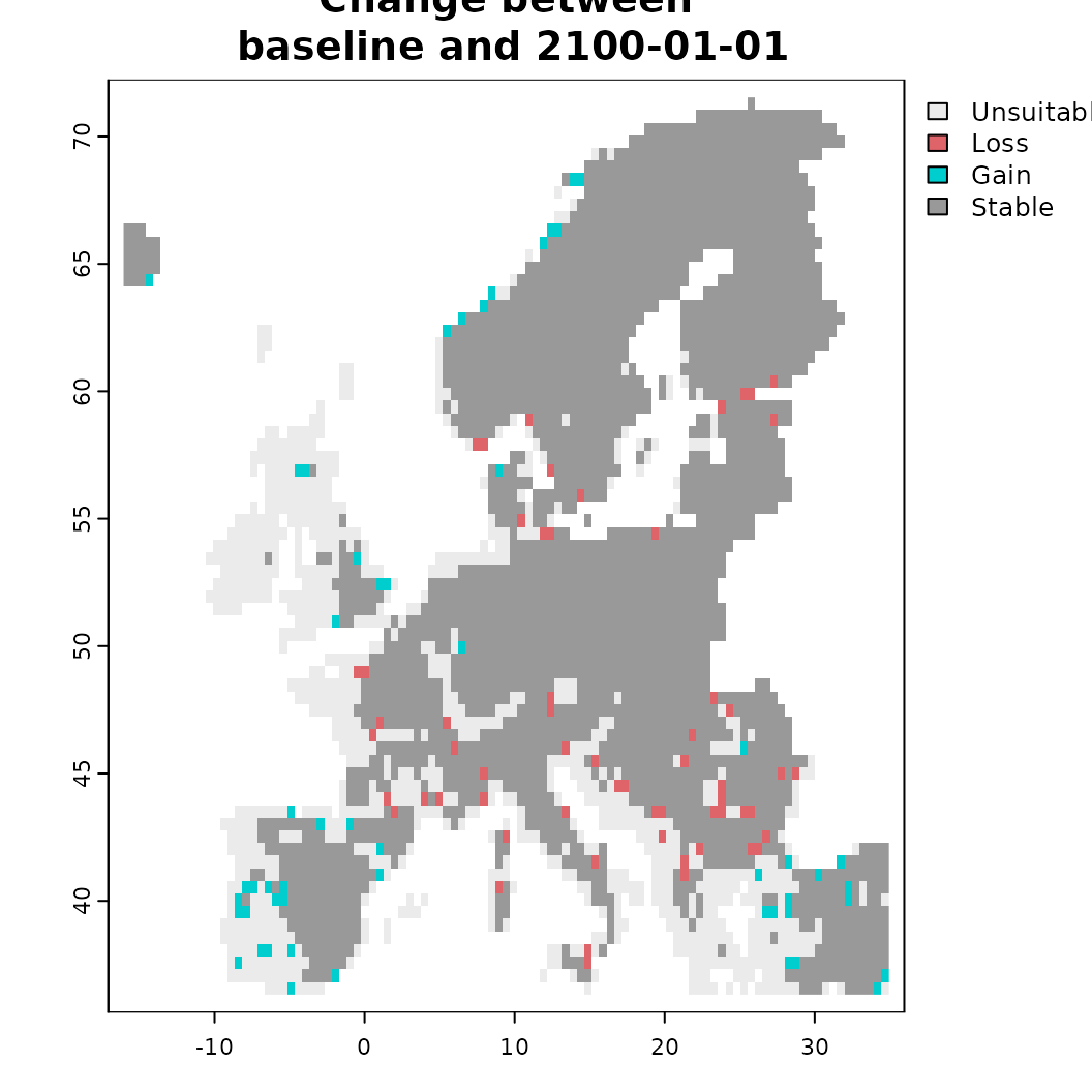
# We can also summarize the thresholded data
o <- sc.fit1$summary()
plot(area_km2~band, data = o, type = 'b',
     main = "Suitable habitat across Time",
     ylab = "Amount of area (km2)", xlab = "Time")
# How does habitat gain and loss change over time?
plot(totchange_gain_km2~band, data = o, type = 'n',
     main = "Habitat gain and loss", ylim = c(-1.5e4, 1.5e4),
     ylab = "Amount of area (km2)", xlab = "Time")
lines(o$totchange_gain_km2~o$band, col = "blue")
lines((o$totchange_loss_km2)~o$band, col = "red")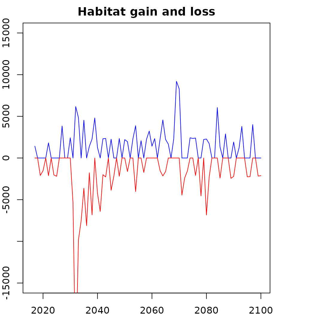
Finally, scenarios projections can also be saved as specific outputs.
As before, this is enabled via write_output() and works
just the same for [BiodiversityScenario] objects, with the
only difference being that the output can be specified as netCDF-4
file.
Adding constraints to projections
In the simple scenario above we use the naive assumption that any,
depending on the response functions of the fitted distribution model,
any suitable habitat within the background modelling region is
potentially reachable by the species. In reality there might however be
geographic (e.g. islands), environmental and biotic constraints on how
far a species can disperse. These can be specified through the constrain
function [add_constraint()] and a variety of constraints is
currently available, some of which depend on other packages.
-
add_constraint()Generic wrapper to which a specific ‘method’ can be supplied. See documentation for more information on available options and parameters. -
add_constraint_dispersal()To add a dispersal constraint to the projections which is applied after each time step. Supports various options with'sdd_fixed'for fixed dispersal kernels,'sdd_nexpkernel'for a negative exponential kernel or'sdd_kissmig'for applying the kissmig framework. -
add_constraint_MigClim()Use the MigClim R-package to simulate dispersal events between time steps. A number of parameters are required here and adding this constrain will also overwrite some default plotting capacities (For example viasc$plot_migclim()). See also the help file and Engler et al. (2012) for more information. -
add_constraint_connectivity()Add a connectivity constrain to the projection. Currently only hard barriers are implemented, but in future additional sub-modules are planned to enable more options here. -
add_constraint_adaptability()Simple constraints on the adaptability of species to novel climatic conditions. Currently only simple nichelimits are implemented, which ‘cap’ projections in novel environments to the observed ranges of contemporary predictors. -
add_constraint_boundary()Specifying a hard boundary constraint on all projections, for example by limiting (future) projections to only a certain area such as a biome or a contemporary range.
Lastly there are also options to stabilize suitability
projections via the project() function. Specifying a
stabilization here results in the projections being smoothed and
informed of incremental time steps. This can particularly help for
projections that use variables known to make sudden, abrupt jumps
between time steps (e.g. precipitation anomalies).
# Adding a simple negative exponential kernel to constrain the predictions
sc.fit2 <- sc |>
   add_constraint(method = "sdd_nex", value = 1e5) |>
   # Directly fit the object
   project(stabilize = F)

# Also fit one projection a nichelimit has been added
sc.fit3 <- sc |>
   add_constraint(method = "sdd_nex", value = 1e5) |>
   add_constraint_adaptability(method = "nichelimit") |>
   # Directly fit the object
   project(stabilize = F)

# Note how constrains are indicated in the scenario object.
sc.fit3
#> Spatial-temporal scenario:
#>   Used model: GLMNET-Model
#>  ---------
#>   Predictors:     bio01, bio12, crops, ... (9 predictors)
#>   Time period:    2016-01-01 -- 2100-01-01 (83.9 years)
#>  ---------
#>   Constraints:    dispersal (sdd_nexpkernel), adaptability (nichelimit)
#>   Threshold:      0.03 (percentile)
#>  ---------
#>   Scenarios fitted: Yes

# The naive assumption is that there is unlimited dispersal across the whole background
# Note how the projection with dispersal constrain results in a considerable smaller amount of suitable habitat.
sc.fit1$plot(which = 40) # Baseline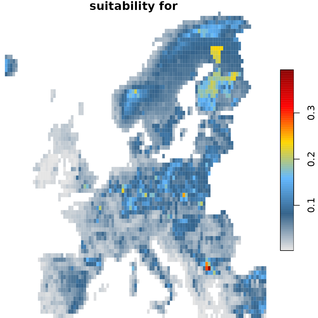
sc.fit2$plot(which = 40) # With dispersal constrain
sc.fit3$plot(which = 40) # With dispersal limit and nichelimitation (within a standard deviation)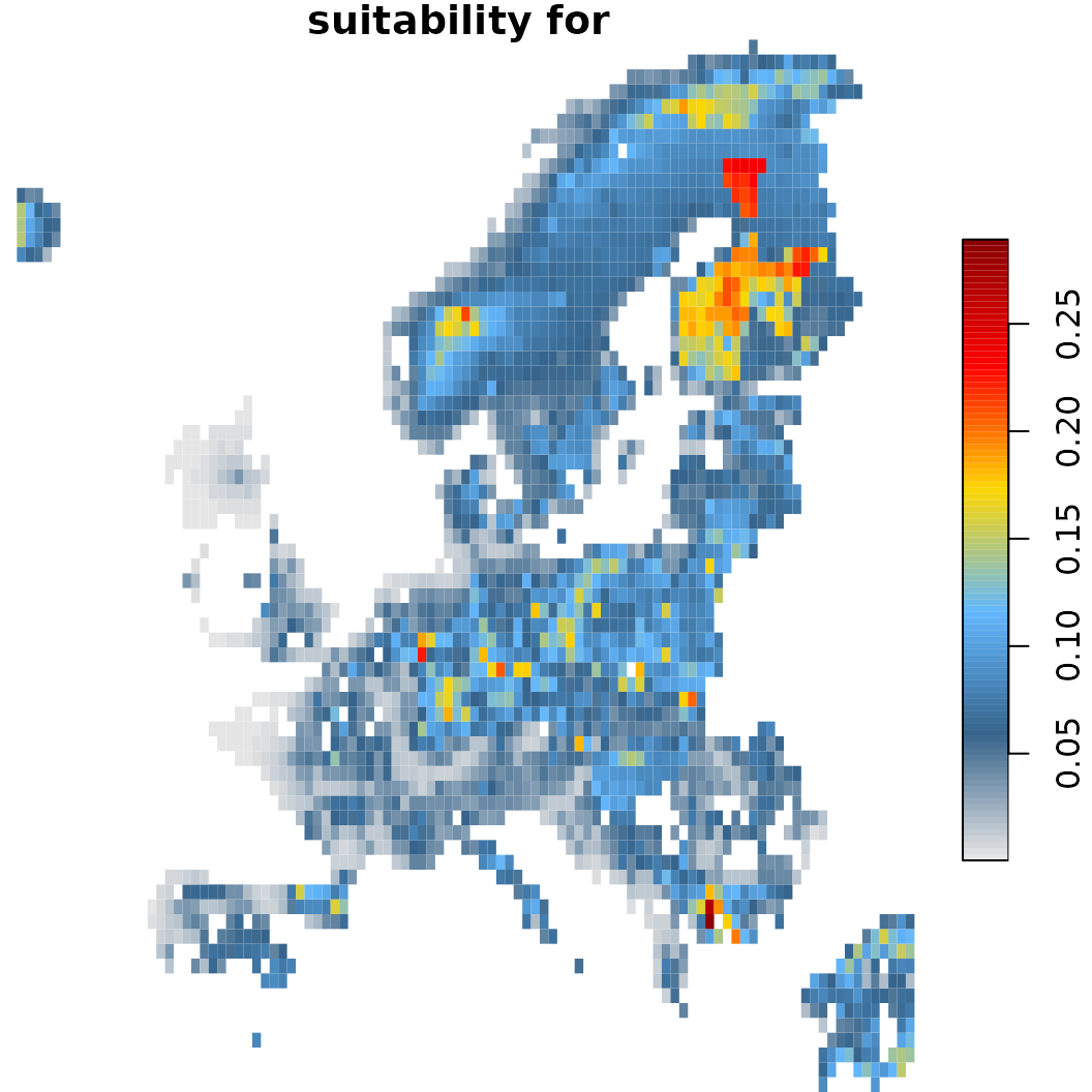
# Lets compare the difference in projections compared to the naive one defined earlier.
o1 <- sc.fit1$summary()
o2 <- sc.fit2$summary()
o3 <- sc.fit3$summary()
arlim <- c(min(o1$area_km2, o2$area_km2, o3$area_km2)-10000,
           max(o1$area_km2, o2$area_km2, o3$area_km2))

plot(area_km2~band, data = o1, type = 'n',
     ylim = arlim,
     main = "Suitable habitat projection",
     ylab = "Amount of area (km2)", xlab = "Time")
lines(o1$area_km2~o1$band, col = "black", lty = 1)
lines(o2$area_km2~o2$band, col = "black", lty = 2)
lines(o3$area_km2~o3$band, col = "black", lty = 3)
legend("bottomleft",
  legend = c("Unlimited dispersal", "Constrained dispersal",
             "Constrained dispersal and niche limit"),
  lty = c(1, 2, 3),
  cex = 1.2,
  bty = "n")
# Lastly it is also possible to directly summarize the state
# before (usually first year) and end (last year).
sc.fit2$summary_beforeafter()
#> # A tibble: 13 × 5
#>    runname    category                  period        value unit
#>    <chr>      <chr>                     <chr>         <dbl> <chr>
#>  1 Simple PPM Current range             2016-01-01 434.     ha
#>  2 Simple PPM Future range              2100-01-01 422.     ha
#>  3 Simple PPM Unsuitable                84 years   188.     ha
#>  4 Simple PPM Loss                      84 years    12.3    ha
#>  5 Simple PPM Gain                      84 years     0.234  ha
#>  6 Simple PPM Stable                    84 years   422.     ha
#>  7 Simple PPM Percent loss              84 years     2.83   %
#>  8 Simple PPM Percent gain              84 years     0.0540 %
#>  9 Simple PPM Range change              84 years   -12.0    ha
#> 10 Simple PPM Percent change            84 years    -6.01   %
#> 11 Simple PPM Sorensen index            84 years     0.987  similarity
#> 12 Simple PPM Centroid distance         84 years    16.4    km
#> 13 Simple PPM Centroid change direction 84 years     4.33   deg
Another option for constraining prediction is also by imposing a
zonal limit (for instance climatically defined) on the projections (see
alternatively add_constraint_boundary() above). This has to
be done while fitting the SDM for the reference conditions (see the
example with limits (1) ) and
is considered when doing (future) projections.
Specific parsers for GLOBIOM related scenarios
IIASA’s Global Biosphere Management Model (GLOBIOM) is a partial equilibrium model and used to analyze the competition for land use between agriculture, forestry, and bioenergy, which are the main land-based production sectors. It builds on.
With the ibis.iSDM being part of IIASA’s suite of integrated models,
there is a direct link available to make use of downscaled GLOBIOM
outputs. Implemented are functions to either directly format the data
via [formatGLOBIOM()] or add them to any
DistributionModel-class or
BiodiversityScenario-class object directly via
add_predictors_globiom() .